So far, in the systems we have discussed, we have assumed that every machine stores all data. In the earlier chapter on replication, when the primary node receives a write request from a client, it saves the entire dataset both locally and on other replica nodes. This storage approach has the following problems:

• Scalability: If data replication is done in a primary-backup manner, all the work falls on the primary node. Under heavy load, the primary node quickly becomes a bottleneck.
• Single-node bottleneck: A single node, due to the physical limits of its hardware (disk, memory, CPU, etc.), will always hit an upper bound on processing capacity.
• Failure isolation: If a node hosting a specific portion of the data fails, that data becomes unavailable, reducing the overall availability of the system. For example, if data from different cities were stored on different nodes, a service outage in one region would not affect data in other regions.

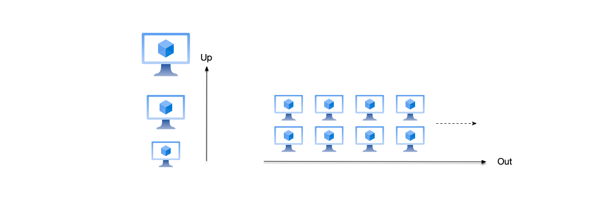
When scaling a system, engineers typically choose between two primary strategies, as illustrated below:

• Vertical Scaling: Also known as “Scale Up,” this improves processing capacity by adding more resources to a single server (e.g., faster CPU, more RAM, larger disk).
• Horizontal Scaling: Also known as “Scale Out,” this distributes the load by adding more servers and forming them into a cluster that works together.

Vertical scaling requires expanding the capacity of only a single node and has the following advantages:

• Simplicity: Managing and maintaining one machine is far simpler than managing a cluster.
• Strong data consistency: All data resides on a single machine, eliminating the need to handle complex distributed data synchronization and consistency issues in distributed systems; transaction processing is simple.
• Low latency: Inter-process communication (IPC) within a single node is very fast with no network overhead.
• Application transparency: Application code usually does not require major changes to adapt to stronger hardware.

However, any machine’s CPU and memory expansion has physical limits and cannot be increased indefinitely. Furthermore, it introduces a single point of failure; a server crash completely halts the service, resulting in poor availability. Maintaining a single node also poses significant challenges, as it typically requires scheduled downtime.

In contrast, horizontal scaling expands the system’s processing capacity by adding machines and has the following advantages:

• Theoretically unlimited scaling: When load increases, you only need to add more standard servers to the cluster, providing excellent scalability.
• High availability and fault tolerance: If one or more servers in the cluster fail, the system can continue to serve (with possible performance degradation) without a single point of failure.
• Cost-effective: A cluster can be built using large amounts of inexpensive hardware, resulting in lower total cost of ownership.
• Elastic scaling: The number of servers can be dynamically increased or decreased based on load, making it particularly suitable for cloud environments.
• In some scenarios, data partitioning is mandatory. For example, if a service is accessed from different continents, countries, or regions, services need to be deployed separately in those locations.

In horizontal scaling, because data is distributed across different nodes in the cluster, it faces the following challenges:

• Architectural complexity: Additional components and technologies need to be introduced, such as load balancers, service discovery, distributed data storage, and configuration management.
• Data consistency challenges: Managing data state across multiple machines and guaranteeing consistency is very difficult—this will be the focus of the subsequent chapter on distributed transactions.
• Network latency: Communication between nodes relies on the network, which has higher latency and is less reliable compared to IPC within a single node.

We have briefly outlined the pros and cons of both vertical and horizontal scaling strategies above. If an application is in its early stages, with predictable user and data growth within the scope of a single node, vertical scaling is recommended. If explosive user growth and unpredictable traffic spikes are expected, horizontal scaling should be prioritized. This chapter mainly discusses horizontal partitioning strategies.

Horizontal scaling in distributed systems introduces the concept of “Partitioning.” Data is distributed across different machines. As shown below, data is split across two different nodes, rather than having all nodes store all data.

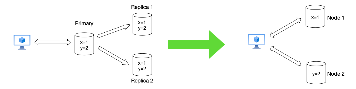
Note that “partitioning” in this context refers to the intentional division of data across multiple nodes, rather than a “network partition” (which implies an unintentional network failure).

In different systems, “partition” has different names; some systems use “shard,” and others use “region.”

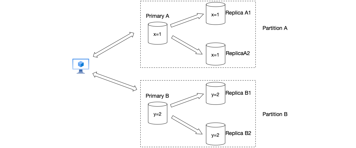
In practice, partitioning and replication are almost always used in tandem. Typically, a single partition is replicated across multiple nodes to ensure high availability and fault tolerance, as shown below.

However, partitioning introduces new complexities:

• How to access data: Previously, you only needed to access the primary node; now you need to consider how to route data requests to the corresponding partition. This is a request routing problem, which we will discuss in depth later.
• Partition rebalancing: One of the goals of partitioning is to distribute data as evenly as possible across multiple partitions. However, when different partitions have uneven data distribution, the issue of partition rebalancing must be considered.
• Global ordering: As we will see, different partitioning strategies have different levels of support for global ordering. If global ordering is a common operation the system needs to consider, a partitioning strategy that is friendly to global ordering should be chosen.

In this chapter, we will discuss the following topics related to partitioning:

• What are the common data partitioning methods and their pros and cons.
• How to route data requests to the corresponding partition, and common strategies for implementing request routing.
• When certain partitions receive high traffic, a partition hotspot problem arises. How should this be solved?
• Finally, as a phased summary of the replication and partitioning chapters, we will examine the implementation plans of several projects.

Partitioning Strategies #

Range Partitioning #

Range partitioning is the most intuitive partitioning strategy in distributed data storage. Its core idea is very simple: treat the data primary key as a continuous ordered sequence, and assign each resulting range to a different node for management.

Imagine a dictionary divided into different volumes based on the first letter of entries:

• Volume 1: Contains entries starting with A–B.
• Volume 2: Contains entries starting with C–E.
• …

This is typical range partitioning. In this analogy, the dictionary words are the partition keys, and each volume is a partition. When you need to look up the word “Apple,” you know it must be in Volume 1; when looking up “Cake,” it must be in Volume 2.

In distributed systems, these “boundaries” are explicitly defined. The system maintains a global routing table, recording the mapping relationships as shown below:

Partition ID	Start Key	End Key	Node
P1	−∞	1000	Node A
P2	1001	2000	Node B
P3	2001	3000	Node B

In real-world applications, range partitioning is typically used for data with natural ordering attributes:

• Time-series data such as monitoring logs, transaction records, and instant messaging messages, where time is chosen as the partition key.
• Geographic data such as food delivery orders and shared bike locations. The GeoHash algorithm is used to convert 2D latitude and longitude into a string, so nearby locations share similar prefixes and are assigned to the same node, making it easy to dispatch orders or find nearby bikes.
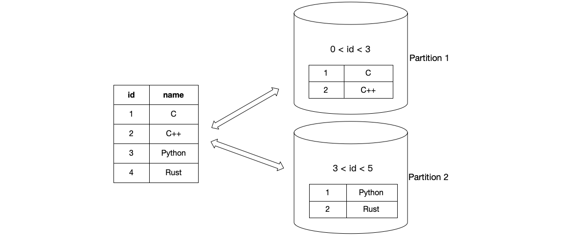
• Business IDs such as user IDs and e-commerce platform order numbers, which usually have auto-increment attributes. The figure below shows an example of using key-value IDs as partition ranges.

The core advantage of range partitioning lies in query performance:

Efficient Range Queries

This is the most prominent advantage of range partitioning. Querying by partition key such as WHERE user_id BETWEEN 500 AND 1500 is very efficient. When performing range queries, the system can quickly determine which partitions contain the target data range, accessing only those relevant partitions rather than all data. This is called partition pruning[1].

Physical Data Locality

Because adjacent keys are stored on the same partition, sequential scans of continuous data (e.g., scanning all data within a certain time period) perform very well, fully utilizing the sequential read/write characteristics of disks.

Easy to Manage and Understand

For administrators, range-based partitioning rules are very intuitive and easy to manually manage and optimize.

---

The primary drawbacks of range partitioning are directly tied to its strengths. Range partitioning divides data based on the ordering of the sequence. If data access patterns are not uniform, it leads to severe load imbalance and hotspot problems. This is called data skew:

Sequential Write Hotspots

If the partition key is an auto-increment ID or a timestamp, all newly written data will have incrementing keys (e.g., 10001, 10002, 10003…). According to range rules, these largest keys will always fall into the last partition. Although the cluster has multiple nodes, only the node storing the current largest key is bearing the write pressure.

In time-series data, the system’s latest data (e.g., logs or orders from the most recent hour) is typically accessed most frequently. If partitioned by day, the “today” partition will bear enormous write and read pressure, while the “last year” partition is almost never accessed, forming a hotspot partition.

Workload-Driven Hotspots

Suppose partitioning is done by user ID range. If a certain range happens to contain a “super VIP” (e.g., a celebrity on social media) or corresponds to an ultra-large enterprise customer (SaaS scenario), this specific partition will become overloaded due to excessive request volume, creating a severe bottleneck for the entire system. Because the partition maps to a physical range, isolating this specific hot ID is notoriously difficult.

Complex Metadata Management

Range partitioning requires a metadata management component (e.g., HDFS NameNode, TiKV PD) to maintain the global routing table. Clients typically query and cache this routing table before reading or writing data. If the routing table changes (e.g., due to splitting), the client’s cache becomes invalid, causing access errors that require retries and metadata updates. We will continue to discuss this problem later in this chapter.

---

To address hotspot and load imbalance issues in range partitioning, the following solutions are available:

Composite Key Design

In the scenarios described above where load imbalance may occur, a single partition key is chosen, such as a timestamp or ID. You should try to avoid choosing keys that will inevitably produce hotspots. If you must choose a key that will produce hotspots as the partition key, consider combining it with other fields to form a composite partition key. This technique strikes a delicate balance between ordering and uniformity. For example, if you must partition by time, consider combining the timestamp with another field (e.g., device ID, user ID suffix). For instance, define the partition key as (user_id_hash, year, month). This ensures data is first partitioned by year and month at a coarse granularity, and then within the same month, data is distributed across different partitions by user_id_hash, avoiding a single partition from becoming too large or too hot.

Pre-partitioning

Based on the expected data distribution, create multiple shards in advance rather than starting from a single shard. This avoids having only one shard bearing all the pressure in the early stages of the system. For example, TiDB supports the pre-split feature[2].

Dynamic Partition Splitting

The system monitors the resource usage of each node. When it detects that a partition’s size or throughput exceeds a threshold, it automatically splits it into smaller partitions.

---

Range partitioning is a powerful and intuitive strategy. It aligns the physical storage of data with its logical order, providing strong performance for range queries and sequential access scenarios. However, its success highly depends on the choice of partition key and access patterns. If hotspot issues cannot be effectively resolved, it can easily become a bottleneck for the system.

Load Rebalancing

When discussing partitioning strategies, in addition to focusing on how data is accessed, attention should also be paid to the load rebalancing performance of different partitioning strategies. This is the core mechanism for maintaining system stability, high availability, and high performance. Simply put, it is the process of migrating data or compute tasks from high-load nodes to low-load nodes when nodes are added, removed, or when the load distribution becomes uneven.

Before diving into the process, we need to understand what situations trigger rebalancing. These are typically divided into passive and active triggers:

• Node addition (Scale-out): A new node joins the cluster and needs to share traffic and data from existing nodes.
• Node contraction/failure: A node goes offline or fails, and its tasks or data need to be transferred to the remaining healthy nodes to ensure replica count and availability.
• Data skew: Certain partitions become very large or receive very high access traffic, becoming hotspots and causing their nodes to be overloaded. Even if the number of nodes does not change, data distribution needs to be adjusted.

Rebalancing must meet the following requirements:

• After rebalancing, the load (data items, write and read requests in nodes) should be evenly distributed among the existing nodes in the cluster.
• When rebalancing data, only data items that need to be migrated between nodes should be moved, saving network and disk I/O load.
• During rebalancing, the system must remain available—it should continue to accept reads and writes.

The essence of rebalancing is re-establishing the mapping relationship between data and nodes, which depends on the underlying sharding strategy. Let’s look at how various partitioning strategies affect data migration.

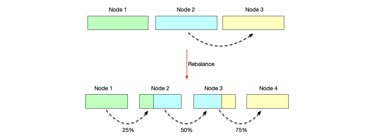
The figure below shows the rebalancing process for range partitioning. Three colors are used to distinguish data originally distributed across three nodes. If the data was originally evenly distributed across three nodes, when a new node is added, each original node should migrate data to the next node in the range: Node 1 migrates 25% of data to Node 2, Node 2 migrates 50% of data to Node 3, and so on. As you can see, during range partitioning rebalancing, every node is affected, just to different degrees.

Hash Partitioning #

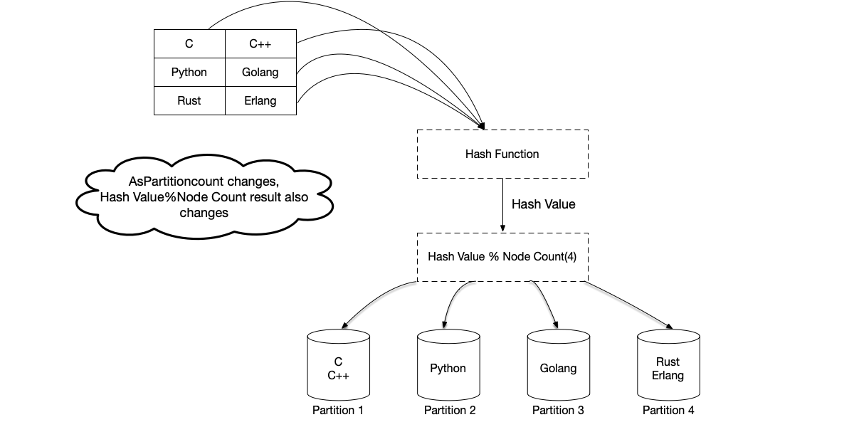
Hash-based Partitioning is another common partitioning strategy. It is a data-agnostic distribution strategy. A hash function takes arbitrary input and produces a fixed-size, random yet deterministic output. Data is assigned to a partition by taking the hash modulo the number of partitions (hash(key) % N, where N is the number of partitions). When choosing a hash function, uniform distribution of data is required. Common algorithms include MD5, CRC32, MurmurHash3, and SHA-256.

Hash partitioning has the following advantages:

• Load balancing: This is the primary goal of hash partitioning. A good hash function can distribute input data evenly across the output space, ensuring that each partition stores roughly the same amount of data and receives a similar volume of requests, effectively avoiding hotspot issues.
• Point query performance: For exact-match queries based on the partition key (e.g., user_id = 7), the system can directly calculate the target partition, achieving O(1) time complexity routing by accessing only a single node.

Because hash partitioning is data-agnostic, it sacrifices ordering for uniformity, facing the following challenges:

Inefficient Range Queries

The hash function destroys the original order of the partition key. A query like WHERE user_id > 1000 becomes meaningless because the hash value’s magnitude is unrelated to the original value. The system must broadcast (scatter/gather) the query to all partitions and then merge the results, which is extremely inefficient and has high latency.

Therefore, if the business frequently requires range queries, hash partitioning should not be the first choice.

Another solution is to design a composite primary key that contains both a hash component and a range component. For example, the primary key can be designed as PRIMARY KEY (country, user_id), where country is the partition key—it is hashed first to determine which partition the data goes to; user_id is the clustering key, responsible for sorting within the partition. This allows efficient queries of WHERE country = 'CHINA' AND user_id > 1000. This query only hits the partition storing Chinese user data and performs an efficient range scan within that partition.

Hotspot Issues Still Exist

Even though hash partitioning provides relatively more uniform data distribution, business-level “super hotspots” can still exist. For example, posts by certain celebrities on social media may attract significantly more attention. This type of problem is called a hot key problem. One solution is to prepend a random prefix (a “salt”) to the original partition key, turning one data item into multiple items distributed across different partitions.

For example, a superstar’s social platform ID user:123 is a hot key. When writing data for this star, instead of writing directly to user:123, write to user:123_salt0, user:123_salt1, … user:123_salt9 (a total of 10 different keys). These keys are distributed across 10 different partitions through hashing. When reading, to retrieve all data for the star, the client must query all 10 keys (user:123_salt*) in parallel and then merge the results in the application layer. The advantage of this solution is that it can effectively distribute the read/write pressure of a single hotspot across multiple partitions. The disadvantage is that it greatly increases read complexity and overhead. Since random suffixes are appended during writes, the exact partition holding the data becomes unpredictable during reads. Consequently, clients must issue parallel queries across all possible suffix variations—a scatter-gather approach that inherently incurs significant overhead. It is a trade-off strategy that sacrifices read cost for write balance.

High Cost of Rebalancing

The naive hash(key) % N approach suffers from a critical flaw: when the number of partitions N changes (nodes are added or removed), the mapping relationship for the vast majority of data becomes invalid. Comparing the hash partitioning figure above with the one below, the number of nodes increases from 4 to 5. Therefore, although the same hash function is used, because the number of nodes has changed, the result of the hash function modulo the number of nodes also changes, causing the same key to migrate to a different machine.

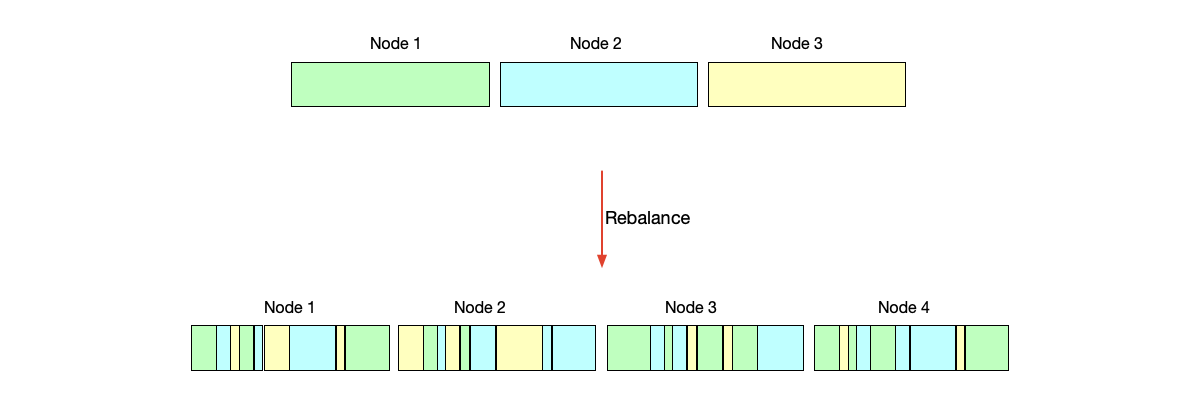
Compared with the load rebalancing process of range partitioning, which requires data continuity, even when rebalancing affects all partition data, the post-rebalancing data distribution is still largely predictable. In contrast, the modulo approach in hash partitioning not only affects all partitions, but the new data distribution also appears chaotic and difficult to predict, as shown below.

Although hash partitioning solves load balancing at the cost of sacrificing range query capabilities, in production-grade distributed storage systems (such as Apache Cassandra), designers do not choose between “hash” and “order.” Instead, they adopt a clever hybrid partitioning strategy.

The core of this strategy lies in introducing a composite primary key, splitting the key into two independent dimensions:

• Partition Key: Responsible for “which machine to go to.” This is the first part of the primary key. The system performs hash calculation on the partition key and distributes data evenly across different physical nodes based on the consistent hash ring. This ensures global load balancing and avoids data skew.
• Clustering Key: Responsible for “how to arrange within the machine.” This is the second part of the primary key. Within the same partition (i.e., the same physical node), data is not stored randomly but strictly sorted by the clustering key’s value (usually stored in an SSTable). This ensures local ordering of data.

Suppose we are designing a “user orders” table where query requirements are typically “query a user’s orders from the most recent six months.” Set user_id as the partition key and order_time as the clustering key. The write and query flows are as follows:

• Write: Data is routed to the corresponding node based on Hash(user_id), but within that node, the user’s orders are strictly arranged by order_time.
• Query: The query first locates the node via the hash algorithm in O(1) time, then performs a highly efficient sequential scan within that node.

This “global hash location, local ordered scan” design perfectly combines the write scalability of hash partitioning with the read flexibility of range partitioning. It is one of the best practices for processing massive time-series data and user-dimensional data.

To address the problem caused by partition count changes in hash partitioning, consistent hashing is introduced.

---

Consistent Hashing #

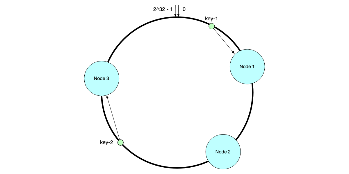
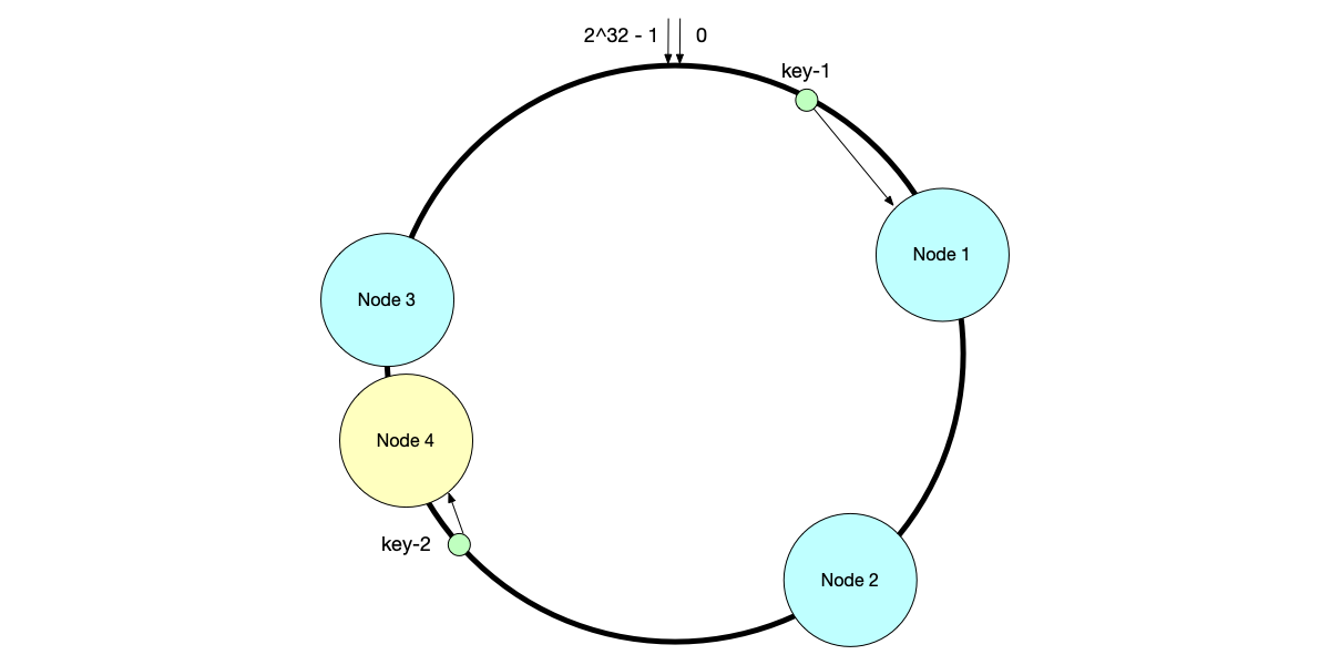
Consistent hashing was first introduced in the seminal paper [3]. Its core idea is: instead of using the node count N as the modulus, a large, fixed hash ring is used as the mapping space. Through the hash ring, both data and nodes are mapped to the same circular space (usually 2^32 − 1). Data keys are stored on the nearest node in the clockwise direction. When reading or writing data, the hash value of the key is calculated and taken modulo the ring size. The first node found in the clockwise direction is the target node.

As shown below, after key-1 is mapped to the ring space, the first node found in the clockwise direction is Node 1, so this record is stored on Node 1. Similarly, key-2’s data is stored on Node 3.

Because the ring size is fixed from the start, the same key will always map to the same position on the ring. When the number of nodes changes, it will only affect data distribution near the added node.

As shown below, after adding Node 4, some data previously written to Node 3 will migrate to Node 4, while data previously written to Nodes 1 and 2 does not need to be migrated.

As shown below, after removing Node 3, requests originally on Node 3 will migrate to the first node in the clockwise direction (Node 1), while other nodes are unaffected.

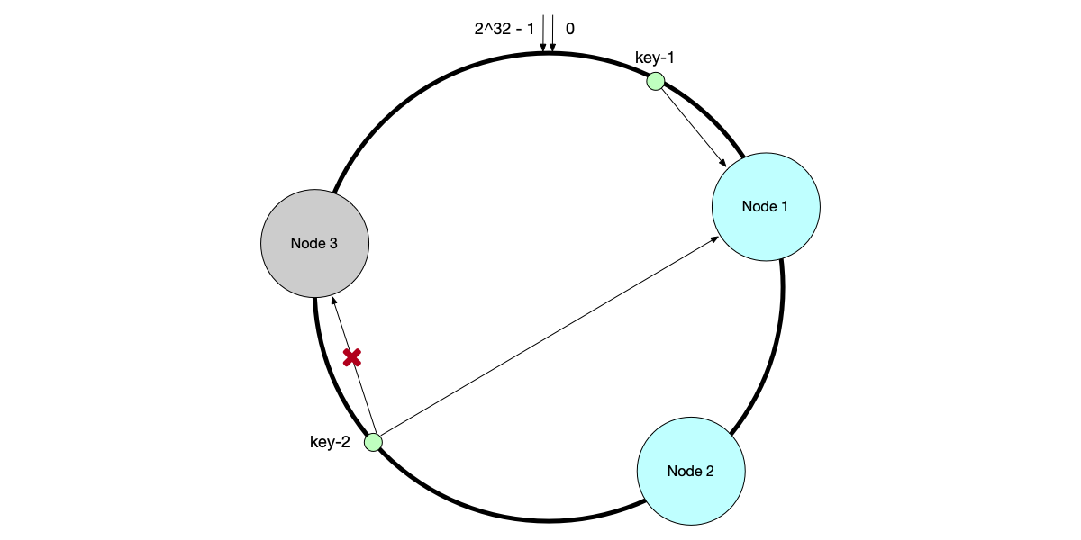
As you can see, when adding or removing nodes, the consistent hashing algorithm only affects data on a portion of the nodes on the hash ring; other data is unaffected.

However, standard consistent hashing also has its own disadvantages:

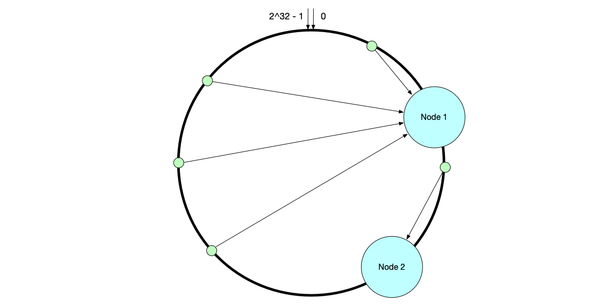
• Load imbalance: The consistent hashing algorithm cannot guarantee uniform distribution of data on the hash ring, which may lead to access skew with large amounts of data concentrated on a few nodes. As shown below, due to uneven data distribution, Node 1 bears a large amount of access.
• Load imbalance during node changes: When a node goes offline, all data it was responsible for will be transferred entirely to its next node. This newly responsible node suddenly has to bear the data volume of two nodes, easily triggering a cascading failure. Similarly, when adding a node, it only relieves pressure on its next node; other nodes are unaffected and the load remains uneven.
• Ignoring node heterogeneity: Some nodes have better machine performance and should handle more requests, while others with poorer performance should handle less. However, the current design maps all physical nodes to a single point on the hash ring regardless of performance.

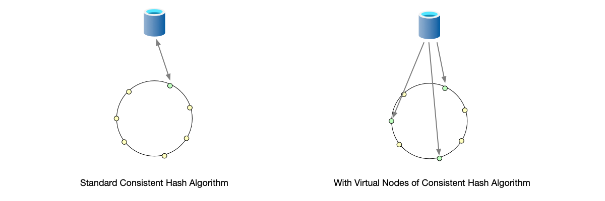
To solve this problem, the industry generally adopts a variant of consistent hashing [4]. As shown below: each physical node is no longer mapped to a single point on the ring, but to multiple points (i.e., multiple virtual nodes):

• When data is mapped to the hash ring, it is no longer mapped to physical nodes but to virtual nodes.
• Each physical node manages multiple virtual nodes.
• Considering the different performance of physical nodes, different physical nodes may manage different numbers of virtual nodes.

As shown below, the system has only two physical nodes. Physical Node 1 manages virtual nodes [A1, A2, A3], and Physical Node 2 manages virtual nodes [B1, B2, B3]. The number of virtual nodes is three times the number of physical nodes, and data distribution is more uniform.

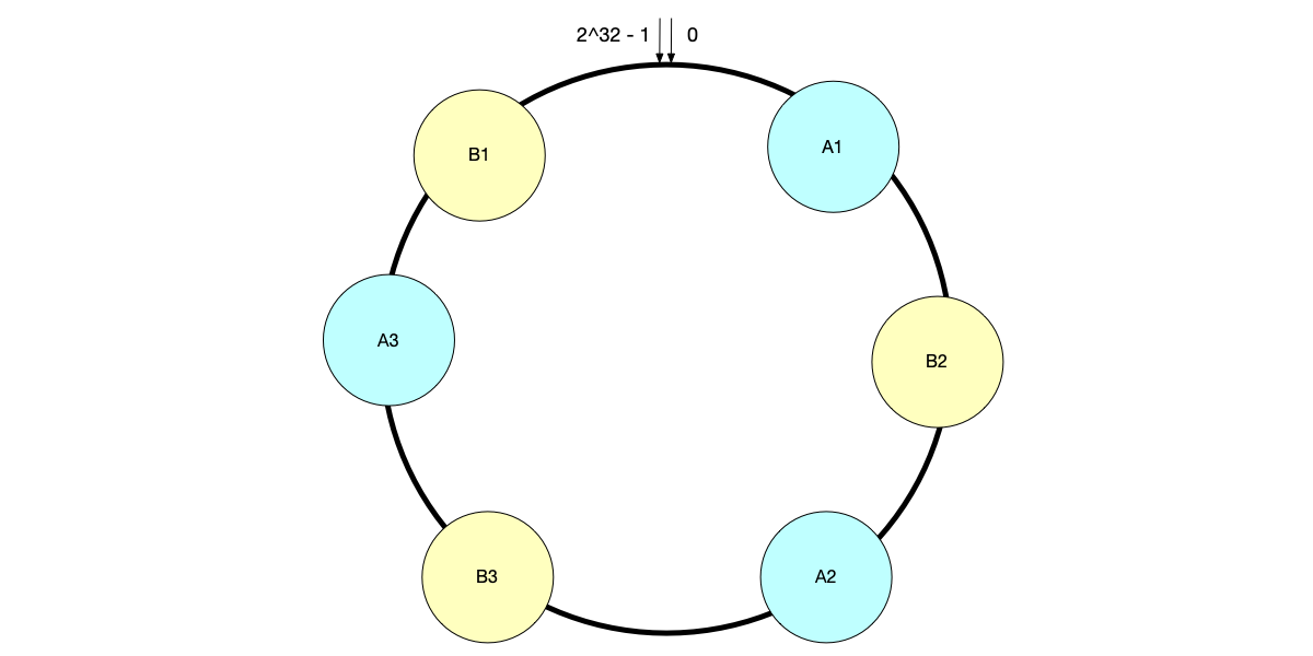
Introducing virtual nodes brings the following benefits:

• Load balancing: Because each physical node has a large number of virtual nodes scattered around the ring, data items on the ring will be more evenly handled by different virtual nodes, and therefore distributed more uniformly across physical nodes. The more virtual nodes there are, the more uniform the load becomes. By increasing the number of virtual nodes, load distribution can be smoothly optimized. All of this greatly improves load balancing among physical nodes in the system.
• Graceful degradation during node failures: When a physical node fails, its workload is not shifted entirely to a single contiguous successor. Instead, its virtual nodes fail simultaneously, and their data is redistributed across multiple successor virtual nodes belonging to different physical nodes. The data originally managed by these virtual nodes will be evenly transferred to other virtual nodes on the ring, which belong to multiple different physical nodes. This means the data load is evenly redistributed to all remaining physical nodes rather than crushing a single node, effectively preventing cascading failures.
• Convenient adjustment of node weights: If certain physical nodes have stronger performance (e.g., better CPU, memory, disk), you can allocate more virtual nodes to them. Nodes with stronger performance have more virtual nodes, meaning they occupy more intervals on the ring and can bear a larger proportion of data volume and traffic, achieving weighted load balancing.

The comparison between standard consistent hashing and consistent hashing with virtual nodes is shown below. Currently, almost all production systems that use consistent hashing for partitioning (such as Redis Cluster, Dynamo, etc.) adopt consistent hashing with virtual nodes.

Feature	Standard Consistent Hashing	Consistent Hashing with Virtual Nodes
Load Balancing	Poor, prone to hotspots	Excellent, more virtual nodes means more uniform
Node Failure Impact	May cause downstream node overload, triggering cascading failures	Smooth, load shared by all surviving nodes
Flexibility	Low, all nodes have the same weight	High, weights adjustable via virtual node count
Implementation Complexity	Simple	Slightly complex, needs virtual-to-physical mapping

Hash partitioning is a strategy that pursues data distribution balance as its core goal. By sacrificing range query capabilities, it gains unparalleled load balancing characteristics and efficient point query performance.

The core challenge and key innovation of its technical evolution lie in rebalancing, and the implementation of consistent hashing with virtual nodes elegantly solves this problem, making it the de facto standard partitioning scheme for modern distributed systems (especially key-value stores and caches). Choosing hash partitioning means you are very certain that your workload consists of a large number of random point queries and has extremely high requirements for load balancing.

Data Migration Process #

We have already discussed the load rebalancing processes of different partitioning strategies. This section discusses the data migration process, which not only occurs during rebalancing but also during node repair, replica replenishment, cross-datacenter synchronization, and other scenarios.

In the replication chapter, we discussed the data replication process. While they share overlapping underlying mechanisms, they differ fundamentally in their purpose, lifecycle, and trigger conditions.

• Data replication is a normal, continuous process whose purpose is to maintain data redundancy. As long as the system exists, this process continues. In many cases, data replication is a one-to-many process (e.g., in primary-replica replication, the primary node replicates data to multiple replicas).
• Data migration is more of a temporary process that is only initiated when data needs to be moved. It is generally a one-to-one process.

Because of this difference, data migration involves not only moving data but also determining when to switch requests from the source node to the new node. Data replication does not have this process.

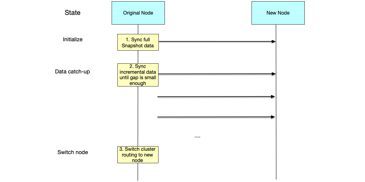
As shown below, the general data migration process is as follows:

1. Initialization: Synchronize the full snapshot data to the new node.
2. Catch-Up: Synchronize new data written after the full snapshot to the new node.
3. Switch node: When the data gap between the source node and the new node is small enough, complete the cluster routing table switch. The new node officially takes over all requests. This switching process will affect system availability.

In the migration process, the final routing table switch is a difficult point. It faces the following challenges:

• During the switching gap, there may be brief periods of service unavailability. For example, first stopping writes to the source node and waiting for the new node to confirm it has caught up before updating the routing table. This catch-up takes some time, during which write requests may return errors.
• After updating the routing table, propagating the metadata information takes some time. During this process, clients may still believe the source node is active and continue writing data to it.
• In addition to these challenges, there may also be residual clients that maintain long connections with the source node. Even after the routing table has been updated, they continue sending requests to the source node.

To address these issues, we propose the following solutions.

Blocking Switch

This is the safest solution but results in brief system unavailability. It is suitable for scenarios with extremely high consistency requirements that can tolerate millisecond-level jitter. The process is as follows:

1. Disable writes to source node: After the source node receives the switch command, it rejects all new write requests and only processes read requests.
2. Catch up final data: The new node catches up the last newly written data.
3. Configuration change: After the new node catches up, update the routing table to perform the switch.

Version-based Request Fencing

The Fence mechanism mentioned in the replication chapter can be used for protection:

1. Each node maintains a monotonically increasing version number. During switching, the source node increments the local partition’s version number.
2. When the old node continues to receive client requests, due to the version number mismatch, the old node can either forward to the new node or reject the client’s request, prompting it to update the route and retry.

This solution solves the “routing delay” and “connection residue” problems. Old requests are intercepted and will not cause data pollution.

Seamless Dual-Write and Read

This is the most complex solution but is imperceptible to users. It is suitable for database-level migration or cross-datacenter migration. Its mechanism introduces an intermediate state where the system requires a log to be committed only when it is durably written to a majority of both the old and new configurations.

This solution ensures that even if both the source node and the new node want to be the leader at the same time, they must get approval from the other configuration. It is impossible for both to succeed simultaneously. This achieves smooth transition without stopping writes. The process is as follows:

1. Enable dual-write: When old and new node data is sufficiently close, the client (or proxy layer) sends write requests to both the source node and the new node simultaneously.
2. Source as authority: At this time, reads still go through the source node. The new node’s data is only used for “warm-up” and verification.
3. Seamless switch: Once data consistency is confirmed, simply modify the read routing in the configuration center to point to the new node, then disable dual-writes (routing all writes exclusively to the new node). This method can achieve true “zero downtime,” but the client implementation complexity requirement is extremely high.

We will deeply explore Raft’s joint consensus membership change algorithm in the consensus algorithm chapter. This algorithm is an implementation of the dual-read dual-write idea.

The above solutions make trade-offs between “availability” and “consistency.” Through the standard paradigm of “catch up data → brief write blocking → change metadata → resume writing,” we can achieve absolute data consistency guarantees with minimal availability loss (millisecond-level blocking).

Request Routing #

In both the replication and partitioning chapters, the same type of problem is involved: how does a client’s access reach the corresponding node?

• In the primary-replica replication model, write requests need to be sent to the primary node.
• In data partitioning, data needs to be sent to the corresponding node.

This type of problem is commonly called request routing. This section will summarize the most common types of request routing implementations. As we will see, the primary distinction among these implementations lies in where the routing logic resides.

Because the request routing discussed here includes both primary node processing of client write requests in primary-replica replication and data processing by the corresponding partition node in data partitioning, for simplicity, in the following descriptions, saying a node can process a client request means:

• In primary-replica replication, the node is the primary node.
• In data partitioning, the node is the partition where the data resides.

Request Routing Patterns #

There are three request routing patterns: server-side proxy, client-aware, and independent routing layer. The difference between these patterns is: who bears the responsibility for request routing. We will discuss them in order.

Server-side Proxy Pattern

As shown below, in this implementation, the client does not need to know any partition information. All nodes are equal, and each node maintains a routing mapping table. Therefore, the client can connect to any node to send requests:

• If the node can process the request, it processes it and responds to the client.
• Otherwise, the node forwards the request to the node that can process it, receives the response, and then responds to the client.

This pattern completely decouples the client from the cluster topology. The client remains utterly agnostic to partition boundaries or primary-replica roles, allowing for a lightweight (or “thin”) implementation, using a generic protocol to access it. The disadvantage is that forwarding requests may result in an extra hop.

Smart Client Pattern

In the other two routing patterns, besides knowing how to access nodes or routers (domain names, IP addresses, ports, etc.), the client knows nothing else about the nodes (e.g., whether it is a primary node, which partitions’ data it can process, etc.). In other words, in the first two approaches, node information is “transparent” to the client. Besides these two approaches, the client can also be aware of node information, so it knows which node to access from the start.

As shown below, compared to the first two approaches, the client implementation in the smart client pattern is “heavier.” In this implementation, besides request-response logic, the client also needs to maintain node information itself. For example, when nodes change, the client needs to update this metadata in real time; when requests are rejected, it needs to implement its own retry logic. In this mode, complexity is pushed down to the client. Therefore, clients in this pattern are also called “smart client.”

Therefore, in client-aware approaches, an SDK is generally provided for users. This involves potentially implementing multi-language versions of the SDK to meet user needs. In the first two approaches, if the request protocol is a generic protocol (e.g., HTTP), a generic protocol client can be used. Additionally, in the smart client pattern, because there is no network hop and clients connect directly to nodes, performance is relatively higher. Projects such as Kafka and ZooKeeper adopt the fat client pattern.

Independent Routing Layer Pattern

As shown below, in this approach, the client does not communicate directly with nodes but first connects to a routing layer. The routing layer is responsible for parsing protocols, maintaining routing tables, and forwarding requests. When receiving client requests, it does not process them but forwards them to the corresponding node for processing.

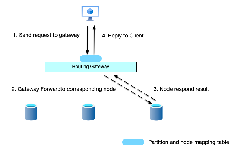
The advantage of the routing layer pattern is that it decouples the business layer from the access layer. The business layer can scale freely without the client being aware, and routing rule changes are entirely handled in the access layer. In the server-side proxy pattern, if the receiving node is not the target processing node, an extra hop occurs. However, the routing layer pattern will always have one extra hop.

We have analyzed the pros and cons of several pattern implementations. Before choosing a request routing pattern, the following questions need to be considered:

• Latency sensitivity: If the business is very sensitive to latency and cannot accept even one extra network hop, then client-aware is the only choice.
• Client diversity: Is multi-language client access needed (Java, Go, Python, Rust…)? If there are many client languages, maintaining a client for each language is extremely costly because you have to rewrite complex routing logic for each language. In this case, a middle proxy or server-side routing is more suitable.
• Connection management model: Is the business long-connection or short-connection? If there are massive short connections, clients directly connecting to backend storage nodes may exhaust their file handles. Introducing a routing layer to do connection pooling is a good defensive measure.
• Architecture decoupling: When backend scaling occurs, is client restart or upgrade allowed? If not, the dumber the client, the better. Hide complexity inside the routing layer or nodes.

The table below compares these patterns.

Dimension	Smart Client Pattern	Server-side Proxy Pattern	Independent Routing Layer Pattern
Network Hops	1 hop (direct)	1 or 2 hops (may require inter-node forwarding)	2 hops (routing forwarding)
Client Complexity	High (fat client, needs routing logic)	Low (thin client, only needs to connect to any node)	Low (thin client, only needs to connect to router)
Ops Complexity	Low (no extra components)	Medium	High (needs to maintain extra routing cluster)
Coupling	High (client needs to be aware of topology changes)	Medium (client aware of cluster, not partitions)	Low (client completely unaware)
Connection Pressure	Storage nodes bear all client connections	Storage nodes bear connections	Routing layer bears connections
Multi-language Support	Difficult (need complex SDK for each language)	Easy	Easy

Request Routing Implementation #

Regardless of which routing pattern is adopted (client-aware, proxy forwarding, or routing layer), the system’s core challenge is how to maintain and propagate partition metadata.

Partition metadata refers to the global mapping relationship that records “which data partition is stored on which physical node.” Unlike stateless services that only need to know “which nodes are alive,” distributed storage systems must precisely know “which node manages Key X.”

In industry practice, there are typically two mainstream implementation solutions:

External Consensus and Coordination Service

This is the most common and architecturally clearest solution. The system introduces a highly available external coordination component (such as ZooKeeper, etcd) or a dedicated metadata management node (such as HDFS NameNode, TiDB PD) to maintain the global routing table.

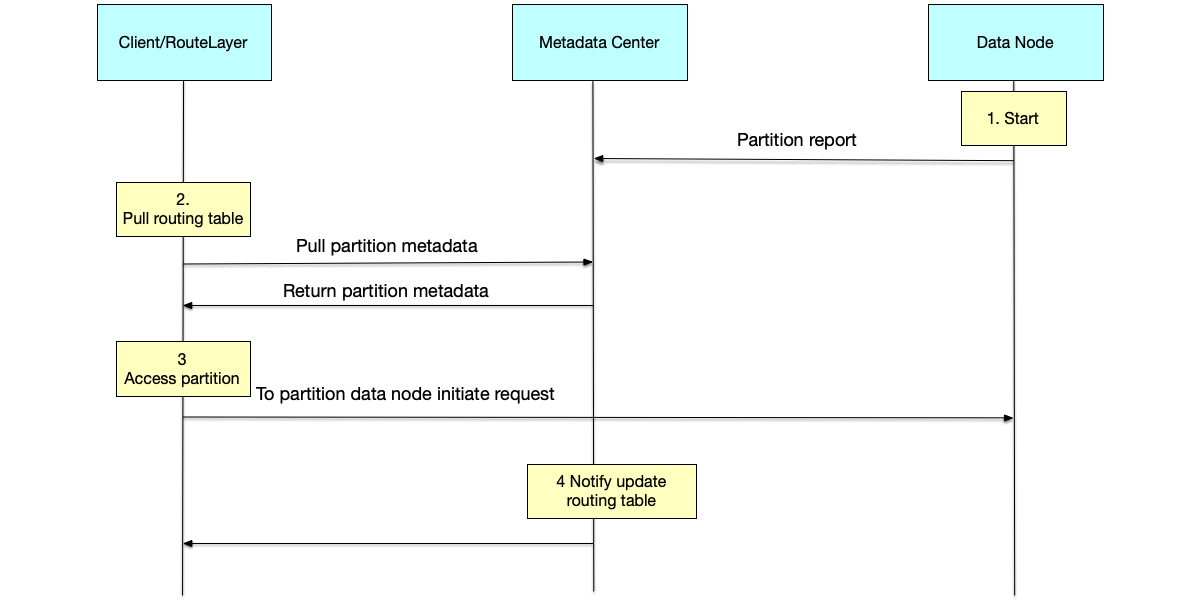
As shown below, its workflow is typically as follows:

1. Registration and reporting: When a data node starts, it registers with the metadata center the partition ranges it is responsible for. When data migration (rebalancing) occurs, nodes also report the latest partition ownership.
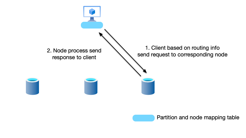
2. Subscription and notification: When a client (or routing layer) starts, it pulls the complete partition mapping table from the metadata center and caches it locally.
3. Local routing: When a client initiates a request, it only needs to locally compute the key’s hash value or range, consult the cached mapping table to locate the target node, without querying the coordination component for every request, thus ensuring high performance.
4. Updating routing table: In addition to the above process, when the routing table changes, clients also need to be notified. Clients typically subscribe to changes via a Watch mechanism. Once metadata changes, clients can perceive them in real time and update their local cache.

The advantage of this solution is single source of truth; metadata consistency is easy to guarantee. The disadvantage is the introduction of additional external dependencies. If the coordination component completely fails, although it does not affect established reads and writes, it prevents the cluster from scaling or recovering from failures.

Metadata for request routing is typically maintained using a strongly consistent model. We will discuss how to implement a consensus algorithm that satisfies the strongly consistent model in the consensus algorithm chapter.

Gossip Protocol and Decentralized Routing

To avoid the single-point risk of centralized components, systems represented by Cassandra and Redis Cluster adopt a decentralized approach.

In this solution, there is no central node with a global observer in the cluster. Each data node saves a cluster routing table from its own perspective, and nodes periodically exchange status information through the Gossip protocol.

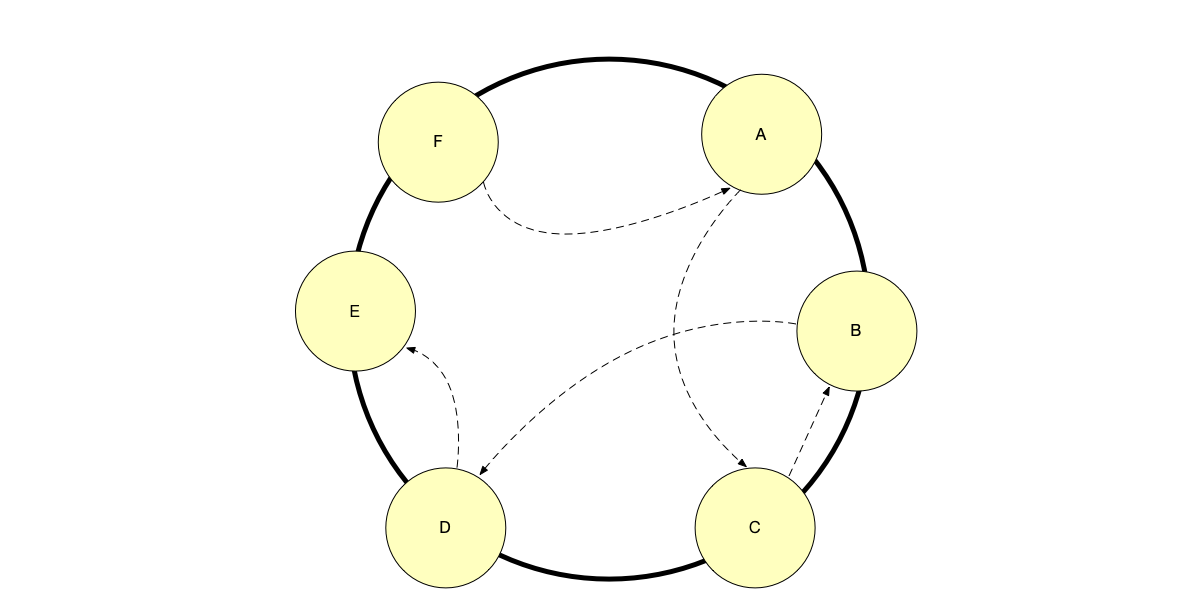
The Gossip protocol workflow is as follows:

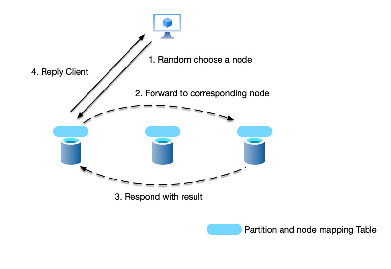
1. State propagation: A node randomly selects another node and informs it of the latest routing information, as shown below. This state information propagates epidemically throughout the cluster, and eventually all nodes converge to a consistent global routing view.
2. Client requests: Clients can send requests to any node in the cluster.
3. Smart forwarding:
   • If the receiving node happens to hold the data, it processes it directly.
   • If the data is not on that node, the node informs the client based on its routing table: “The data is on Node C, please redirect” (e.g., Redis’s MOVED response); or acts as a temporary proxy, forwarding the request and returning the result to the client (e.g., Cassandra).

The advantage of this solution is extremely strong scalability and availability with no single-point bottleneck. The disadvantage is that when the topology changes dramatically, because new routing information is propagated node by node, there can be network storms and slow convergence. Routing tables on different nodes may be temporarily inconsistent, causing clients to need multiple hops to find the correct node. Another important point is that the entire process only satisfies eventual consistency, and it is unknown when the routing data will fully converge. When nodes change dramatically, systems like Redis Cluster may experience large numbers of MOVED or redirects, causing client performance jitter. This engineering cost is often overlooked.

Stale Routing Recovery Mechanism

Regardless of which of the above solutions is adopted, the client’s cached routing table may become stale due to network delays and other reasons. Therefore, mature distributed systems design a set of error correction mechanisms: when a client requests Node A based on an old routing table, if Node A discovers it no longer holds the data (which may have been migrated to Node B), it does not blindly process the request but returns a specific error (e.g., NotMyKey or EpochMismatch). After receiving such an error, the client forcibly triggers a metadata refresh, re-pulls the latest routing table, and retries. This is the last line of defense to ensure system accuracy in dynamic environments.

Chapter Summary #

As data volumes and workloads scale exponentially, single-node storage will eventually hit physical limits in storage capacity, computing power, and network bandwidth. In this chapter, we deeply explored partitioning—the core technology for distributed system scaling. It is the key means to achieve horizontal scaling (scale out), improve system throughput, and increase availability.

In this chapter, we focused on the following core topics:

1. Partitioning Strategy Selection and Trade-offs

Partitioning algorithms determine the distribution of data in the cluster. There is no “one-size-fits-all” strategy; there is only the choice best suited to the business scenario:

• Range partitioning: Preserves key ordering and is extremely suitable for range queries and time-series data, but faces severe “sequential write” and “access hotspot” challenges, which need to be mitigated through careful pre-partitioning or dynamic splitting.
• Hash partitioning: Pursues ultimate data balance, sacrificing range query capability in exchange for uniform load distribution.
• Consistent hashing: Introduces hash ring and virtual node mechanisms, elegantly solving the problem of violent data jitter during cluster scaling, and has become the de facto standard for modern distributed caching and key-value storage.

2. Addressing Data Skew and Hotspots

Theoretical uniform distribution is often broken by the “long-tail effect” of the real world. We analyzed the causes of data skew and access hotspots and proposed application-layer solutions such as composite primary key design and hot-key salting, finding a balance between write balance and read complexity.

3. Data Migration in Dynamic Environments

Distributed systems are not static. We dissected the data migration process during node scaling, failure recovery, and load rebalancing. A robust migration mechanism must minimize impact on online services while ensuring data consistency. We discussed the standard paradigm from full snapshots to incremental catch-up to atomic routing switches.

4. Request Routing Mechanisms

The last mile of partitioning is how to let clients find data. We compared three classic routing patterns:

• Client-aware: Optimal performance but high client complexity and coupling.
• Server-side proxy: Minimal client but adds network hops.
• Independent routing layer: Architectural decoupling, suitable for large-scale microservice systems.

Finally, we compared different implementation schemes for maintaining partition metadata consistency through external consensus and coordination service or Gossip protocols.

Partitioning decomposes massive datasets into manageable subsets, but this is merely the first step. When data is split across different nodes, how do you perform atomic transaction commits across partitions? How do you ensure data consistency among multiple replicas? These new challenges introduced by partitioning will be the foundation for our subsequent discussions on “distributed transactions” and “consensus algorithms.” Through this chapter’s study, we have laid a solid foundation for building highly scalable distributed systems.

---

References #

1. Oracle. Partition Pruning. https://docs.oracle.com/en/database/oracle/oracle-database/21/vldbg/partition-pruning.html
2. PingCAP. TiDB Split Region. https://docs.pingcap.com/tidb/stable/sql-statement-split-region/
3. David Karger et al. “Consistent Hashing and Random Trees: Distributed Caching Protocols for Relieving Hot Spots on the World Wide Web.” Proceedings of the Twenty-Ninth Annual ACM Symposium on Theory of Computing, 1997.
4. Ion Stoica et al. “Chord: A Scalable Peer-to-peer Lookup Service for Internet Applications.” Proceedings of the 2001 ACM SIGCOMM Conference, 2001.