In distributed systems, data replication is one of the core design strategies. Its primary purpose is to improve system reliability, availability, performance, and fault tolerance by redundantly storing identical copies of data:

• High Availability: If only a single node provides service, a single-node failure will render the service unavailable. By replicating data across multiple nodes, even if one node fails, other nodes can continue to provide service.
• Fault Tolerance and Disaster Recovery: Hardware failures, network partitions, or data center disasters can lead to permanent data loss. Multi-copy storage (e.g., cross-rack or cross-region replication) ensures that data is recoverable.
• Reduced Latency: The physical distance between users and data centers causes access latency (e.g., when accessing cross-border services). Replicating data to geographically distributed nodes allows users to access the nearest replica.
• Read Performance Optimization: A single node can become a bottleneck for read requests. Multiple replicas can distribute the read load to improve read performance.

Based on whether a primary node is involved in replication, replication is divided into primary-backup replication and leaderless replication. Primary-backup replication means there is a central node in the system responsible for coordinating write operations and replicating them to other copies. Correspondingly, leaderless replication is a decentralized architecture.

Although data replication brings many advantages, it also introduces the challenge of consistency among multiple replicas due to replication delays. The introduction of data replication brings scalability and reliability, but it also poses the challenge of ensuring semantic consistency across multiple copies. We will delve into the characteristics and implementations of different consistency models. Consistency models vary in their implementation complexity, and different business scenarios adopt different consistency models. We will see that weaker consistency models often suffice for many business requirements.

Note: In many cases, a single node is insufficient to hold all the data of a system. In such situations, data needs to be partitioned across different machines according to certain rules. In this chapter, we assume that a single node has enough capacity to hold all the data of the system.

Primary-Backup Replication #

To ensure high availability of the system, data must be stored on multiple nodes. Every node that stores a complete copy of the data is called a replica. In primary-backup replication, replicas have unequal status and are divided into two categories:

• Primary node: The client’s write requests are first sent to the primary node. After receiving the write request from the client, the primary node saves it to local storage.
• Backup node: After saving the client’s write data locally, the primary node synchronizes the data to the backup nodes. The data on the primary and backup nodes will maintain a strictly consistent write order.

Note: In different systems, the primary node is referred to by different names, such as primary, master, leader, etc. Backup nodes are also referred to by different names, such as secondary, replica, slave, follower, etc.

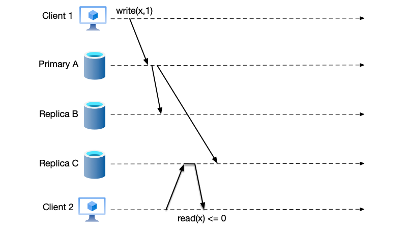
The figure below shows a simple distributed system using primary-backup replication. In primary-backup replication mode, data written to the system must first pass through the primary node and then be replicated to the backup nodes. Unlike write operations, which must go through the primary node, some systems allow read operations to be served by backup nodes. In this case, stale or expired data may be read, depending on the consistency requirements of the system.

Data Replication Modes #

In the figure above, we deliberately ignored a question: when the client writes data, when should the system respond that the write is successful? Is it sufficient to respond after the data is written to the primary node, or should the system wait until the data is successfully replicated to the backup nodes? Based on different response timings, replication modes are divided into: synchronous replication, asynchronous replication, and semi-synchronous replication.

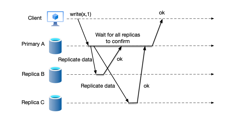
Synchronous Replication

In synchronous replication, the primary node only returns a success response to the client after synchronizing the data to all backup nodes and receiving acknowledgments from all of them. The pros and cons of this mode are as follows:

• Advantages: High data consistency, no risk of data loss.
• Disadvantages: The system’s response time is determined by the slowest backup node. If one node in the system fails or has high network latency, it will affect the success and latency of writes. System availability decreases as the number of backup nodes increases.

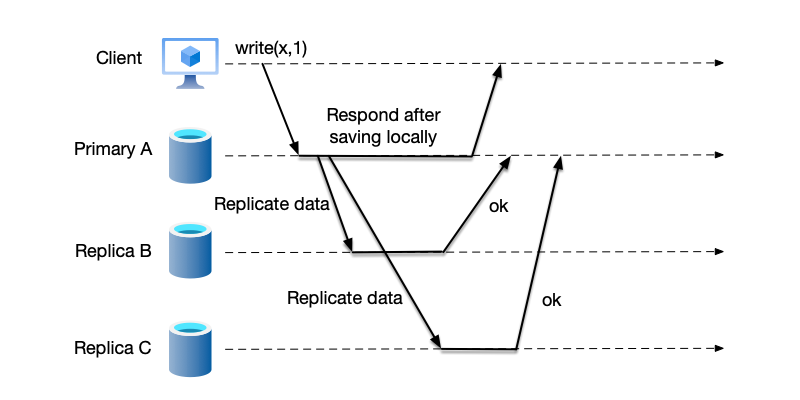
Asynchronous Replication

Completely different from synchronous replication, in asynchronous replication, the primary node can respond to the client with a write success as soon as the data is persisted locally, without waiting for the data to be successfully replicated to the backup nodes. The pros and cons of this mode are as follows:

• Advantages: Low write operation latency, fast client response. The primary node is not affected by backup node failures or network issues, so system availability is high.
• Disadvantages: Weak data consistency, there may be brief inconsistency between the primary and backup nodes. If the primary node fails before the data is successfully replicated to the backup nodes, the unsynchronized data will be lost.

Semi-synchronous Replication

As seen above, both synchronous and asynchronous replication have their drawbacks. The industry more commonly uses a compromise between the two: semi-synchronous replication [1], as shown in the figure below. In this scheme, the primary node does not immediately respond to the client with a write success after saving the data locally, nor does it wait for all backup nodes to replicate successfully before responding. Instead, it strikes a balance: the primary node waits for enough backup nodes to acknowledge the write success.

Under this compromise, because the system only needs to wait for some backup nodes to acknowledge success, it is not affected by the slowest backup node. Therefore, unlike in synchronous replication, the slowest backup node directly determines the system’s response time. Additionally, since data has been replicated to some backup nodes, unlike in asynchronous replication, a primary node failure will not lead to complete data loss.

As for what constitutes enough backup nodes, different systems with different consistency requirements have different needs.

The table below summarizes and compares the working principles, advantages, and disadvantages of the three replication modes.

Mode	Working Principle	Advantages	Disadvantages
Synchronous Replication	The primary node must wait for all backup nodes to confirm receipt and successful write of the data before responding to the client.	Strongest data consistency, ensures data is safely stored on multiple copies.	Very high latency, worst write performance. The failure of any backup node will render the entire system unable to write (low availability).
Asynchronous Replication	The primary node responds to the client immediately after completing the local write, and then asynchronously replicates the data to the backup nodes.	Extremely low latency, best write performance.	High risk of data loss. If the primary node fails before the log is sent, the acknowledged write operations will be permanently lost, causing data inconsistency.
Semi-synchronous Replication	A compromise. The primary node only needs to wait for enough backup nodes to confirm receipt of the data before responding to the client.	Achieves a good balance between performance and data safety.	Still higher latency than asynchronous replication, and if the only acknowledged backup node fails, it degrades to synchronous mode.

Quorum #

When we adopt semi-synchronous mode for data replication, we need to answer a question: how many replicas must the data be replicated to before the system can respond to the client that the replication is successful? In distributed systems, quorum refers to: the minimum number of nodes that must participate and vote in favor for an operation (read or write) to be acknowledged as successful by the system. Generally, a quorum is defined as more than half of the nodes in the system. The quorum mechanism is the rule used to constrain data replication behavior, and it determines the level of replication consistency.

Note: Although in distributed systems, a quorum is usually chosen to be more than half of the nodes in the cluster, commonly known as a majority, a quorum does not necessarily have to be a majority. The core of the quorum mechanism is that the read quorum set and the write quorum set must overlap, but this mechanism is not limited to majority quorums; other quorum mechanisms also exist [2]. For simplicity, in the subsequent descriptions in this book, we will not distinguish between “quorum” and “majority.”

When replicating data, the number of backup nodes that the primary node writes to and waits for acknowledgment from is the “Write Quorum” in primary-backup replication. We use $N$ to denote the total number of nodes in the system, and $W$ to denote the write quorum size, requiring $W > N/2$, meaning the write operation must be acknowledged on more than half of the nodes.

The rationale behind the majority requirement is that distributed systems must reach a unique consensus within the cluster in certain situations. In addition to replicating data, quorums are also used to elect primary nodes. During election, it is necessary to ensure that two primary nodes do not appear simultaneously. When system nodes vote for a candidate primary node, it is mandatory that only a node receiving more than half of the votes can win the election. This guarantees that two primary nodes cannot appear at the same time (because it is impossible for two nodes to simultaneously receive more than half of the votes).

The different data replication modes mentioned earlier can be seen as adopting different quorum settings:

• Synchronous replication: $W=N$, meaning the write operation requires acknowledgment from all nodes before responding.
• Asynchronous replication: $W=1$, meaning the write operation only needs to be replicated to the primary node to respond.
• Semi-synchronous replication: $W > N / 2$, meaning the write operation needs to be replicated to more than half of the nodes before responding.

Note: The quorum mechanism is mainly used to reach a unique consensus in distributed systems, such as replicating data and electing primary nodes. Therefore, it is not only used in primary-backup replication but also in leaderless replication.

Client Request Routing #

In primary-backup replication, the client’s write requests can only be handled by the primary node. Therefore, how the client perceives the primary node becomes a problem. Several common mechanisms exist (for simplicity, the following examples assume a synchronous replication mode).

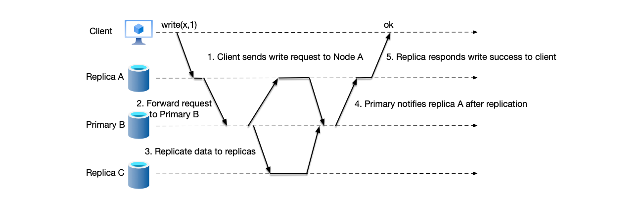
If the node that receives the write request is a backup node, the backup node can forward the request to the primary node. The primary node processes the request and then responds to the backup node that received the client’s request, and the backup node responds to the client with a write success. The figure below is a typical flow chart of forwarding a write request to the primary node:

• Backup node A receives the client’s write request.
• Since backup node A is not the current primary node of the system, it forwards the request to primary node B.
• After receiving the write request, primary node B replicates the data to two backup nodes A and C using synchronous replication mode.
• After completing synchronous replication, primary node B responds to backup node A that the data write is complete.
• Backup node A responds to the client that the data write is successful.

It is worth noting that: the primary node information cached by the backup node might be outdated, meaning the request could be forwarded to a node that is no longer the primary. In this case, the old “primary node” can continue to forward the request to the node it considers to be the primary node. This process continues until the real primary node receives the write request. Generally, all nodes in the system need a mechanism to perceive the switching of the current primary node. For example, in the K8S architecture, the metadata of the running system is stored in etcd. Services that care about cluster changes listen for changes through etcd’s watch API [3].

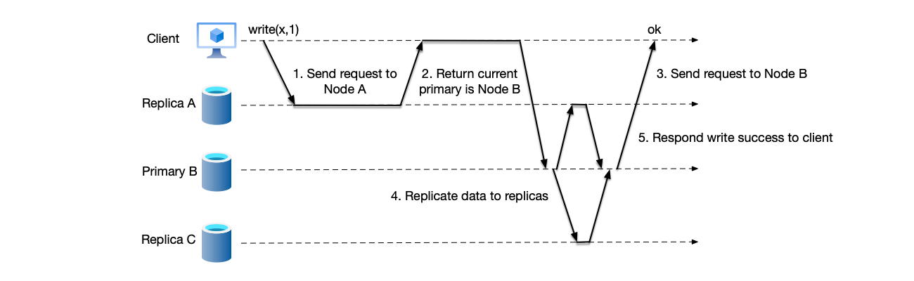
Another method is similar to the previous one. In this method, after receiving the client’s write request, the backup node does not forward the request to the primary node. Instead, it returns the current primary node’s address to the client, and the client retries sending the request using the returned address:

• Backup node A receives the client’s write request.
• Since backup node A is not the current primary node of the system, it returns the address of the current primary node B to the client.
• The client resends the write request to primary node B.
• After receiving the client’s write request, primary node B replicates the data to backup nodes A and C.
• After completing data replication, primary node B responds to the client with a write success.

Alternatively, clients can periodically pull or subscribe to cluster metadata, allowing them to route write requests directly to the appropriate node.

Among these mechanisms, the first is the simplest because the client remains agnostic of the primary node’s identity and requires no additional logic. The disadvantage is that if the client frequently sends write requests to backup nodes, the entire process incurs an additional delay of forwarding from the backup node to the primary node. In the other two methods, the client has to do some extra work. Generally, services that use this type of request method provide an SDK to the client, which encapsulates details such as how to retry and maintain cluster information. However, this also means that some generic clients (such as HTTP protocol) may not be able to simply access the service.

---

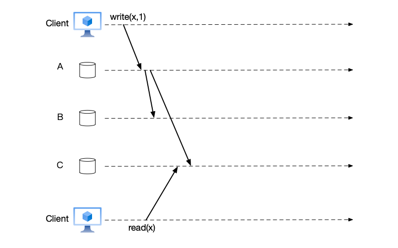
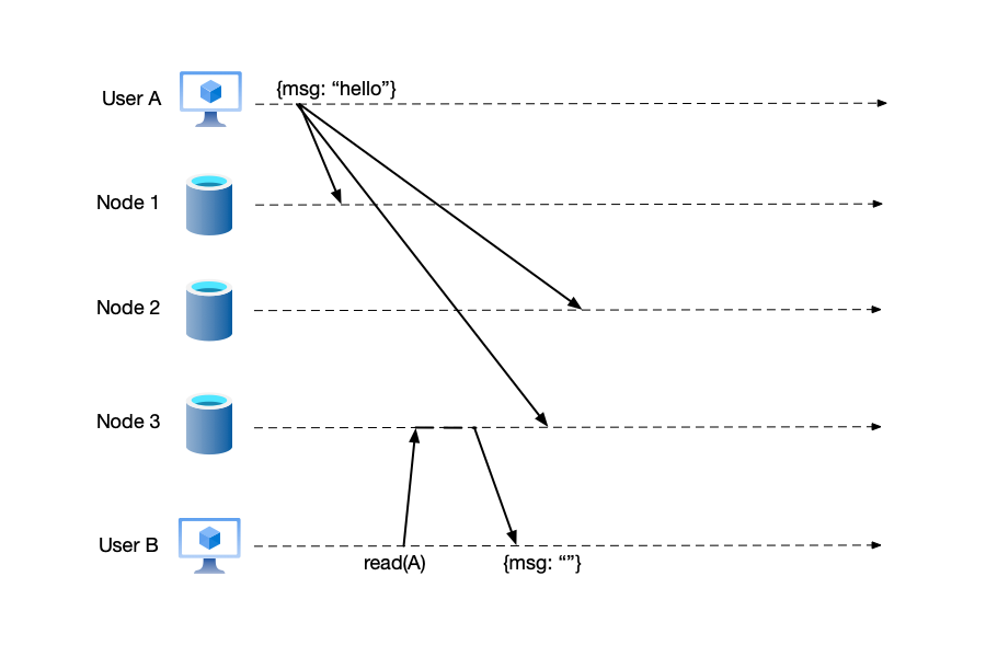
It is worth mentioning that write requests must go through the primary node, while read requests can be handled by any node. However, if a read request is sent to a backup node, the data read may not be the latest. As shown in the figure below, under the quorum mechanism, the write is considered successful, but the client that sent the read request reads an old value. This depends on what consistency guarantees the service provides to the outside world.

Replicating Data #

Previously, we discussed the modes of data replication. In this subsection, we discuss the content of the data being replicated. Recall that a system’s data is divided into the following three categories:

• State: The values of all data in a system. State changes with events.
• Event: Operations that can change the system’s state. In a service, all write requests (writes, updates, deletions, etc.) can be called events.
• Snapshot: A snapshot is a special kind of state. A snapshot is a static state. Once the time of the snapshot is determined, the content of the snapshot is also determined.

Among the above three types of data, which type is used as the content for replication between replicas? The answer usually depends on the delta (or state difference) between the replica’s data and the system’s current latest data.

Among these three types of data, state data and snapshot data are full, static data with a relatively large data volume, while event data is incremental, dynamic data. Therefore, depending on the stage the replica is in, different types of data will be synchronized.

Generally, a newly added node has no data. Catching up to the system’s current state can be challenging because clients continue to write data concurrently while the new node joins. Additionally, if the newly added node cannot immediately catch up to the system’s progress, it may also affect system availability.

• The primary node generates a snapshot of the current latest data and synchronizes this snapshot to the newly added backup node.
• After the snapshot data synchronization is completed, the primary node continues to send the incremental data logs generated after the snapshot to the backup node.
• After completing the previous two steps, the primary node continues to synchronize the data written by the client thereafter to the backup node, until the newly added backup node catches up to the latest data progress of the primary node.

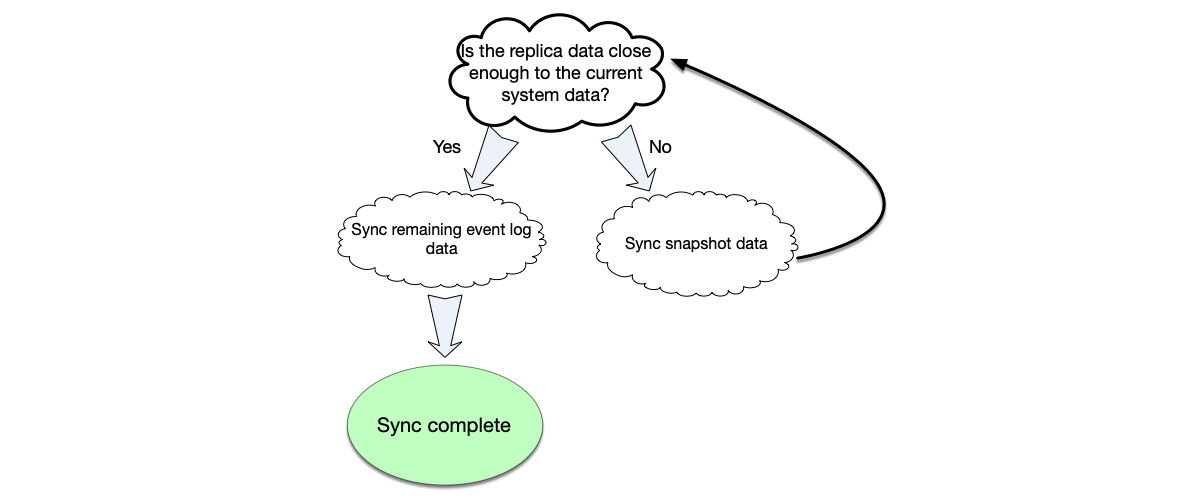
If the data on the replica is very close to the current latest data of the system, the replica can be updated directly by synchronizing incremental event data.

The figure below illustrates the general process of synchronizing replica data. If after synchronizing the snapshot data, it is found that the gap with the current latest data of the system is large again, snapshot data synchronization needs to be performed again until the gap is relatively small before switching to event data synchronization.

This explains the criteria for choosing between snapshots and event logs during data replication. When replicating event data, because event data is data that dynamically changes the system’s state, another factor needs to be considered: determinism. In distributed systems, maintaining the same execution order of events across different replicas is crucial. The same event execution order ensures the system’s determinism. However, the system’s determinism requirements go beyond just the event execution order. Strictly speaking, a system’s determinism requires that its processing of events isn’t timing dependent [4]. In other words: the same event must produce the same result no matter when it is executed.

As shown in the figure below, although the same sequence of events is executed in the same order, due to the $z=\text{random()}$ operation within it, different results will be obtained when executed at different times, leading to system non-determinism.

To summarize, system determinism requires both that events be executed in the same order and that the execution result of each event not depend on time.

According to this standard, let us look at the data content in events. For general KV-type storage (such as Redis, Memcache), it is relatively simple. The content of events is operations that modify specific keys. However, for relational database products, special attention is required.

In statement-based replication, the relational database sends each SQL statement involving database changes (such as Insert, Update, or Delete statements) to the replica for execution. Its advantage is that it does not need to record the changed data of each row, reducing data volume and improving performance. However, its problem lies in non-determinism. If the SQL statement includes non-deterministic statements, such as obtaining random numbers, calling the NOW() function to get the current date and time, UUID() to generate random UUID values, etc., it will lead to inconsistent data across different replicas.

In addition, there is row-based replication. It does not record the executed SQL statements; it only needs to record what a row of data has been modified into. Its disadvantage is the large data volume. For example, for an update statement that modifies multiple records, the modification of each row will be recorded.

MySQL supports both statement-based replication and row-based replication, as well as a mixed mode of the two. For generally side-effect-free statements, statement-based replication is used; otherwise, row-based replication is used.

Node Failures #

In distributed systems, node failures are common. Node failures may be caused by the node itself, such as physical disk or memory exhaustion, code logic issues leading to abnormal exits, or external network issues causing the node to be inaccessible.

Regardless of the cause, when a node fails, at the system level, it manifests as requests sent to the node failing or no longer receiving messages from the node.

In single-node systems, the operating system can accurately determine whether a process has ended. However, in distributed systems, accurately distinguishing between “node crash” and “network delay” in an asynchronous network is theoretically impossible. Therefore, in engineering practice, “absolutely accurate” detection is not performed; instead, timeout-based heuristics are employed, balancing accuracy and completeness. Let us explain the relevant mechanisms for detecting node failures in detail.

Heartbeat is the most commonly used and intuitive fault detection method. There are usually two modes:

• Push mode: The node being detected sends heartbeat messages to the detector at fixed intervals. If the detector does not receive heartbeat messages from the detected node for several consecutive heartbeat cycles, it determines that the detected node has failed. This mode is adopted by most distributed systems.
• Pull mode: Opposite to the push mode, in the pull mode, the detecting node actively initiates heartbeat messages, requiring the detected node to respond. This mode is usually only suitable for scenarios with a small number of nodes.

However, configuring the heartbeat mechanism involves several trade-offs. For example, how long should the heartbeat timeout be set? How many missed heartbeat messages should be considered a node failure? It is possible that the network suddenly jitters, or the node blocks on some time-consuming operations (disk IO, GC, etc.) during runtime, causing the heartbeat message to be delayed, and thus being incorrectly judged as failed. If a node is deemed failed but later resumes operation, it can cause severe availability issues.

The heartbeat mechanism has a fatal problem: inconsistent cluster views. The detector believes that the detected node is down due to network issues and starts to elect a new primary node for failover (selecting a new primary). However, the detected node is actually still alive and believes that it is still the primary node, continuing to write data. This leads to split-brain. As shown in the figure below, due to network issues, node A cannot send messages to node B, causing node B to believe that node A is offline and elect itself as the new primary node. On the other hand, node A believes that it is still working as the primary node. Thus, two primary nodes appear in the system simultaneously.

Distributed systems adopt the lease mechanism to solve this type of problem. A “lease” is a time-limited permit issued by the detecting node to the detected node. The detected node must promise to send a message to the detecting node to renew the lease before it expires. Otherwise, after the lease expires, the detecting node will consider the detected node to be offline. Unlike the heartbeat mechanism, which requires both nodes to send messages to each other, the lease mechanism only requires the detected node to actively renew the lease. This avoids the split-brain problem caused by the detector’s messages failing to reach the detected node due to network issues.

Whether it is the heartbeat or lease mechanism, what is solved is the liveness judgment of one node over another. However, a distributed system is composed of a group of nodes. When replicating data, the same data needs to be replicated across multiple nodes; otherwise, different data may be read from different nodes. Judging node downtime is similar: a single node should not judge a node as down just because its own detection failed. “Judging node downtime,” like “replicating data,” requires agreement among more than half of the nodes. Still taking the split-brain figure as an example, node B judges node A as down because it cannot receive messages from node A, while the communication between node C and node A is normal. At this point, node B and node C have not reached an agreement on the judgment of node A, so node A will not be judged as down and a new primary node will not be re-elected. The election of a new primary node in a distributed system follows a similar process: only when more than half of the nodes have voted for the new node can it be considered successfully elected. Redis adopts the subjective-down and objective-down mechanisms to judge node downtime, which also requires agreement among more than half of the nodes [5].

---

In addition to the mechanism for detecting node failures, after a node fails, there are different handling strategies for primary and backup nodes.

Backup Node Failure

After the primary node detects that a backup node has failed, it will no longer forward client write requests to that backup node. When the backup node recovers from the failure and catches up to the current system progress, the steps are similar to those for adding a new backup node, except that during recovery, data synchronization does not start from scratch.

Primary Node Failure

In comparison, primary node failure in primary-backup replication is more complex because the primary and backup nodes do not have equal status. The primary node is responsible for receiving all client write requests. Therefore, when the primary node fails, a new primary node must be elected. This process is called failover.

• The new primary node is generally elected. The newly elected primary node should ideally have the smallest possible data gap with the original primary node, so that as little data as possible is lost.
• If nodes in the system are located in two different network partitions due to network partitioning, the “split-brain phenomenon” may occur. In this situation, nodes in both network partitions may believe that they are the current primary node of the system and process client write requests. Once the system recovers into a single network partition, the data written on different primary nodes cannot be merged. The split-brain phenomenon causes multiple primary nodes to exist in a system that only allows one primary node at a time, which is a system safety issue and must be avoided.

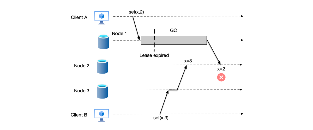
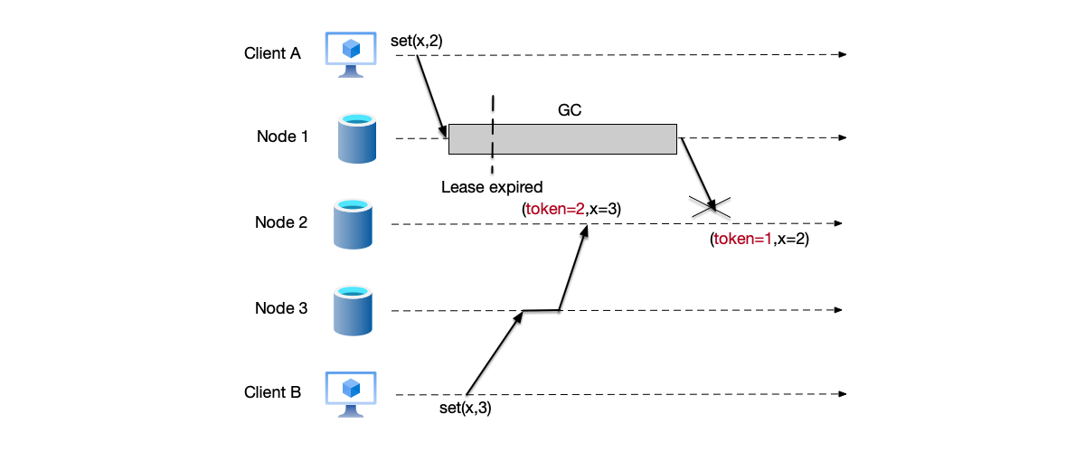
It is particularly important to emphasize that in this subsection, we mentioned using heartbeat and lease mechanisms to detect node failures. However, for primary node failures, these mechanisms alone cannot completely avoid the split-brain problem. As shown in the figure below, the lease mechanism is used to judge the liveness of the primary node. Node 1 is the primary node of the cluster. After receiving the client write request for $x=2$, the lease has not expired and is still valid. However, a Full GC occurs on node 1, causing the primary node term to time out. During this period, node 3 is elected as the new primary node. After this, it receives a client write request for $x=3$ and the write is successful. When node 1 recovers from the GC, it mistakenly believes that it is still the primary node and overwrites the new value with the expired write data $x=2$. This is essentially a “split-brain” problem.

To solve this problem, the system needs a mechanism to determine which node is the current primary node. An intuitive idea is to introduce monotonically increasing version numbers as markers for each primary node. This can distinguish which is the current updated primary node. This method is called fencing token. Every time a new primary node is successfully elected, it receives a monotonically increasing token.

Based on this idea, we revisit the previous scenario, as shown in the figure below. When node 2 receives the data $x=2$ with token=1, because the data $x=3$ with token=2 has already been written previously, the current new primary node’s token is 2. Therefore, it rejects writing the expired data with token=1.

Based on the properties of safety and liveness, looking back at leases and tokens, they solve different problems:

• The role of the lease: it is for the liveness of the system. It ensures that if the primary node really crashes, the system will not be permanently stuck and will be able to elect a new primary node to continue working after some time.
• The role of the token: it is for the safety of the system. It ensures that in the case of “split-brain” or “false death,” the system can only have one legitimate writer, preventing the old primary node from corrupting data.

Leases and tokens must work together to guarantee the safety and liveness of the system.

Note: The token number here needs to satisfy the monotonically increasing property. Essentially, this is a symbol that satisfies the “totality” requirement. When we introduce the implementation of Raft in the consensus algorithm chapter, we will see that Raft’s term number is also a type of token number during primary node election.

Consistency Models #

While data replication brings scalability and reliability, it also introduces a core challenge: how to maintain semantic consistency of data across multiple replicas. This is precisely why we need to systematically study “consistency models.”

Ideally, there should be only one consistency model: after data is updated, all observers immediately see the updated data. If such a guarantee can be achieved, then a distributed system has realized distribution transparency: for users accessing the distributed system, no matter which replica in the system they access, they can read the same data. The distributed system looks like a single system, not a system composed of multiple replicas. In the 1970s, many distributed systems were designed with guaranteeing transparency ahead of system availability [6].

However, by the 1990s, with the rise of large-scale Internet, these practices were re-examined. People began to believe that availability is the most important property of a system. In his 2000 keynote speech on Principles of Distributed Computing, Professor Eric Brewer comprehensively elaborated on different trade-off principles in distributed system design and proposed the CAP theorem on this basis. The theorem states that in a distributed system, the following three properties—data consistency, system availability, and network partition tolerance—can only achieve two at any given time.

In large-scale distributed systems, among the above three properties, network partitioning is a reality that the system must face: distributed systems rely on networks for inter-node communication, and networks are inherently unreliable. Cable failures, switch anomalies, routing jitter, and other factors can all lead to inter-node communication failure. According to the CAP theorem, when network partitioning must be considered, a choice must be made between data consistency and availability. Therefore, consistency and availability cannot be achieved simultaneously. This means there are two different choices in system design: if consistency is prioritized, the system must accept that it may be unavailable at certain times; on the other hand, if the system’s consistency requirements are lowered, the system can continue to maintain high availability when network partitioning occurs.

Regardless of which choice is made, developers need to understand the consistency conditions that the system needs to satisfy. The data consistency mentioned in the CAP theorem refers to linearizability, which is the strongest consistency requirement. However, we will see that in real-world scenarios, there are other available but weaker consistencies that can also satisfy system requirements. In reality, there are different types of consistency, which we call “consistency models.” In this section, we will introduce the most common consistency models. Before doing so, we will illustrate the concept of a consistency model through an example.

Note: This is the first time in this book that we discuss the “consistency” problem. In subsequent chapters, we will also see discussions related to consistency:

• The C in CAP theorem refers to “Consistency,” which is the linearizability discussed below.
• The C in ACID also refers to “Consistency,” but this is a concept more biased toward the database application layer.
• Many people refer to “consensus algorithms” as “consistency algorithms,” but this is actually inaccurate.

What Is a Consistency Model #

When we discussed the order of events earlier, we raised a question, as shown in the figure below:

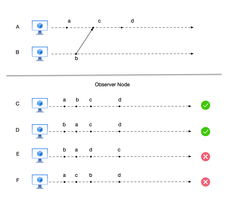
Imagine that in the figure, these nodes are social media accounts. Users C, D, and E follow users A and B. The events at the nodes are the posts of these users on social media. The posts of the followed users will eventually be merged into the followers’ timelines to form a reasonable ordering.

To answer the question of how observers see a reasonable ordering of the followed users’ events, let us first look at the four events on users A and B. According to the Happens-Before relationship, we have:

• $a$, $c$, and $d$ are sequentially occurring events on the same user A. Therefore, $a < c$ and $c < d$.
• First, there is user B’s send event $b$, and then user A’s receive event $c$. Therefore, events $b$ and $c$ have a causal relationship, i.e., $b < c$.
• Finally, according to the transitivity of the Happens-Before relationship between events:
  • $b < c \land c < d \Rightarrow b < d$.
  • $a < c \land c < d \Rightarrow a < d$.

To summarize, for the four events $\{a, b, c, d\}$ occurring on users A and B, the following Happens-Before relationships are satisfied:

$$ \begin{aligned} & a < c \text{, sequentially occurring events on the same user A} \\ & c < d \text{, sequentially occurring events on the same user A} \\ & b < c \text{, events satisfying causal relationship} \\ & b < d \text{, events satisfying transitivity} \\ & a < d \text{, events satisfying transitivity} \end{aligned} $$

From the observer’s perspective, there are $4! (= 4 \times 3 \times 2 \times 1)$ possible ways to order the above four events. However, no matter how they are ordered, the above five Happens-Before relationships cannot be violated.

Based on the above conclusion, we can determine whether the event orderings seen by several observers are correct. The event ordering seen by user E is incorrect because event $c$ occurs before event $d$, but in user E’s event ordering, event $d$ is placed after event $c$. Similarly, the event ordering seen by user F also violates the precedence relationship. The event orderings seen by users C and D differ only in how the two concurrent events $a$ and $b$ are ordered, and in some cases, both are reasonable orderings.

From this example, we can see that in distributed systems, how to have a reasonable ordering of events across multiple nodes is an important problem. The ordering of these events, in addition to being reasonable (e.g., not violating the Happens-Before relationship), is also closely related to the difficulty of system implementation.

Secondly, distributed systems bring conveniences such as fault tolerance and scalability to application developers. The strategies for achieving these conveniences are replication and partitioning. We hope that the same data can always remain consistent across different nodes. However, replication brings a challenge to the system: the consistency problem. When the system replicates data to multiple nodes, there is always a time delay, which creates a risk of data inconsistency.

Requiring a distributed system to guarantee that data on all replicas is always consistent at any moment would come at an enormous cost. Fortunately, it is also not required that all nodes in the system maintain consistent data at all times. It is sufficient for the system to guarantee consistency at the moment when the client reads the data.

The definition of consistency model in Wikipedia [7] is as follows:

In computer science, a consistency model specifies a contract between the programmer and a system, wherein the system guarantees that if the programmer follows the rules for operations on memory, memory will be consistent and the results of reading, writing, or updating memory will be predictable.

When designing a system, knowing what consistency guarantees the distributed system provides is particularly important for application developers. Different strengths of consistency guarantees bring different implementation difficulties and concurrency. Applications determine the required data consistency strength based on the application scenario, for example:

• For some social media message orderings, only causal consistency is required.
• For some critical data that does not allow errors (such as bank deposits, primary nodes in the system, etc.), linearizability is required.

The following uses a social media feed as an example to explain the consistency model issues that need to be considered in system design.

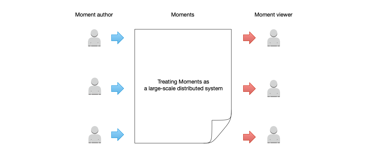
Let us view the social media feed as a large distributed system:

• This distributed system provides write (post updates) and read (browse updates) functions to the outside world.
• This distributed system has two types of clients: clients that post updates are responsible for writing data, and clients that browse updates are responsible for reading data. Of course, often the same client can both read and write.
• The dynamic data is stored on more than one machine. These machines together constitute this large distributed system. Different users do not necessarily write to the same machine when posting updates. Conversely, when browsing updates, they do not necessarily read from the same machine either.

The next question is: can those browsing the feed see globally consistent data? That is, do all people see the updates arranged in the same order?

Many times, even when looking at the comments and replies under the same update, different people do not necessarily see them in the same order. So the answer to the above question is no. This leads to the next question: if different people see the updates (including comments) in different orders, what rules should these orders follow to be reasonable?

Defining these rules is the exact purpose of consistency models.

For a social media feed, an update has multiple people commenting below it. This can be considered a two-dimensional data:

• Process (i.e., the person commenting) is one dimension.
• Time is another dimension, i.e., the chronological order in which these comments appear.

However, from the perspective of readers reading these comments, this two-dimensional data needs to be flattened onto a single dimension of only this process’s timeline, removing the dimension of different processes.

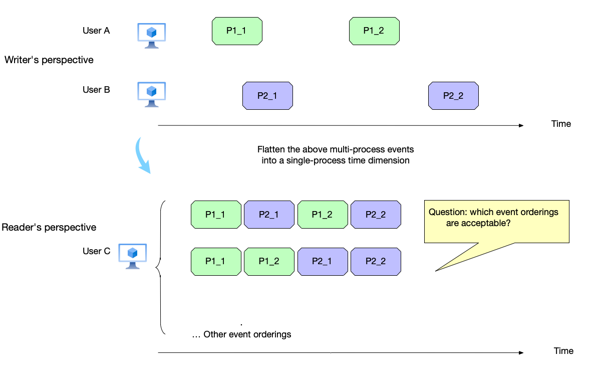
In the figure above, from the perspective of the reading process user C, the events of the two writing processes need to be flattened onto this process’s timeline for arrangement. We can see that these events have multiple possible arrangements after flattening.

Flattening the events of multiple writing processes onto a single timeline is a combinatorial problem. If all the writing process events add up to a total of $n$, then all the permutations and combinations of these events are $n!$. If the current system has events $a$, $b$, and $c$, the different arrangements are: $\{(a,b,c), (a,c,b), (b,a,c), (b,c,a), (c,a,b), (c,b,a)\}$.

A consistency model needs to answer: among all these possible event arrangements, according to the required consistency strictness, which ones are acceptable and which ones are impossible.

---

With these questions in mind, in this section, we will introduce the following common consistency models in order:

• Sequential consistency;
• Linearizability;
• Causal consistency;
• Eventual consistency.

Note: Although eventual consistency is grouped with the other types of consistency models here, we will see later that eventual consistency does not belong to the same concept as these other consistency models.

Consistency Model Diagram Conventions #

Before beginning the introduction of consistency models, it is necessary to first explain the various elements in the consistency model diagrams.

In addition to possible concurrent events on different nodes, events may also overlap in time during execution. In previous diagrams, we used a point on the timeline to represent an event, which created an illusion: events are completed instantaneously. In reality, because each event involves memory reads and writes, CPU computation, disk IO reads and writes, etc., the execution of each event is not instantaneous. When the execution time of events is taken into account, multiple events may overlap during execution.

For clarity, the diagrams in this chapter will no longer treat events as a point on the timeline. Instead, events have two boundaries:

• The invocation time of the event;
• The completion time of the event.

In the diagrams, an event is represented by a rectangle. The left boundary of the rectangle is the invocation time of the event, and the right boundary is the completion time of the event. The width of the rectangle is the execution duration of the event, as shown in the figure below.

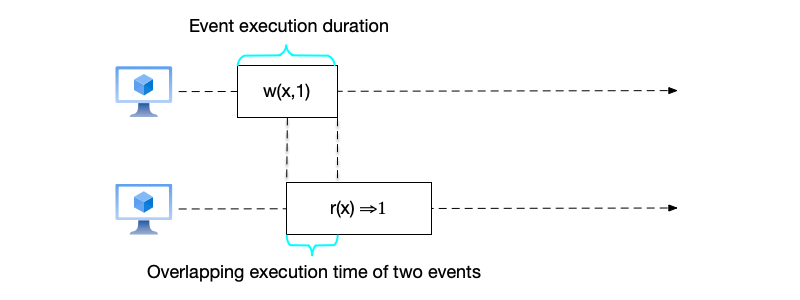
In the figure, there are the following types of operations:

• $w(x,a)$: represents writing data $a$ to variable $x$;
• $r(x) \Rightarrow a$: represents reading variable $x$ with result $a$.

At the same time, if the rectangles of events overlap, it means that the execution times of the two events overlap, and they are considered concurrent events in time. Conversely, if they do not overlap, it means that the events do not overlap in execution time.

Sequential Consistency #

First, we introduce sequential consistency, first proposed by Lamport in the paper [8]:

the result of any execution is the same as if the operations of all the processors were executed in some sequential order, and the operations of each individual processor appear in this sequence in the order specified by its program.

The above definition of sequential consistency can be summarized as: all operations appear to execute in a single global order, and the local operation order of each participant is preserved. It requires the following conditions to be met:

• Events cannot go backward.
• Events within the same node still maintain the same order after reordering.
• The event reordering order that satisfies the above two points is the same in all nodes. That is, the reordered event order is consistent across all nodes in the system.

The following explains these three conditions one by one.

---

First, read operations cannot observe older states. This requirement means: if a new value is written or read, all subsequent events cannot see older data than it. Let us look at an example.

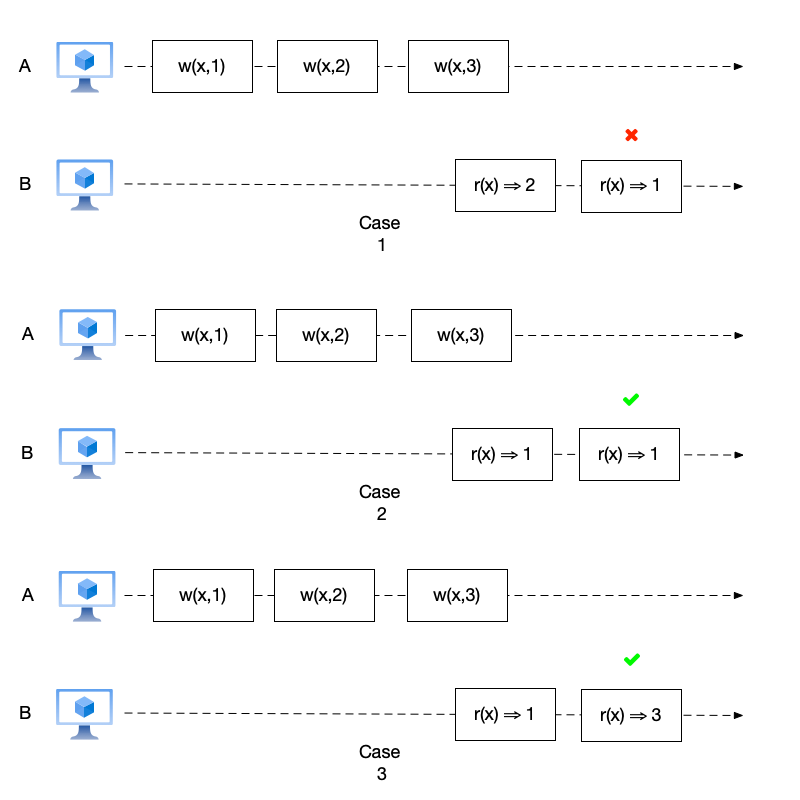
In the three scenarios in the figure above, node A also performs 3 write operations, sequentially writing data 1, 2, and 3 to variable $x$. Node B performs 2 read operations. The prohibition of rollback means that when node B reads, it cannot read an older value than a previous read operation. For example, if it reads $x=2$, then the subsequent read operation cannot read $x=1$, because according to the write operation order on node A, the write operation $x=1$ is before $x=2$.

• In case 1, node B reads $x=2$ for the first time and then reads $x=1$ for the second time. This is an older value compared to $x=2$, so the event has rolled back here.
• In case 2, the second read of $x=1$ is not older than the first read of $x=1$, so this is acceptable.
• Similarly, in case 3, the second read of $x=3$ is also newer than the first read of $x=1$, so it does not violate the rule that events cannot roll back.

Next, let us look at an example of violating the event order on the same node. The event order on node A is $a$, $c$, $d$. However, when reordering events at node E, event $d$ is placed before event $c$. This violates the order of these two events on node A.

Finally, there may be multiple event orderings that satisfy the first two conditions. However, once one is chosen, it must be the same on all other nodes. The reordered order is required to be consistent across all nodes.

Let us try to intuitively understand these requirements of sequential consistency. In an ideal situation, a distributed system should “behave like a single copy.” This actually implies two requirements:

• The system has only one order; otherwise, “a single copy” would be out of the question.
• In addition to the system having only one order, the order also needs to be reasonable. Therefore, it is required to satisfy the event order in the nodes and that events cannot roll back.

---

It should be noted that although several conditions of sequential consistency do not explicitly mention that the event ordering needs to satisfy causality, this point is actually implied in the condition that events cannot roll back. That is, if the result of an event is seen, subsequent events cannot see the cause of the event.

---

With the above basic understanding of sequential consistency, let us look at a few more examples:

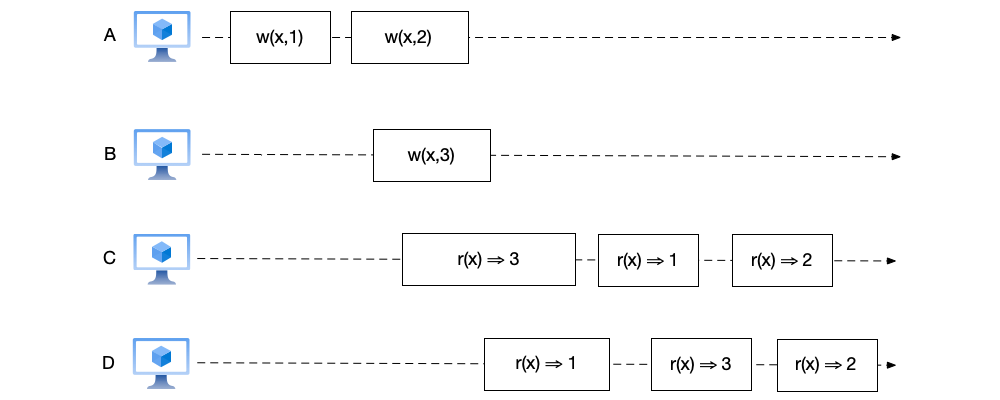
• As shown below, the orders of node C and node D are both reasonable and consistent. They successively read the results of the two write operations on node A, and no event rollback occurs. In addition, for the two concurrent write operations $x=2$ and $x=3$, both nodes also maintain the same read order (first reading $x=2$ and then $x=3$). Therefore, it conforms to sequential consistency.

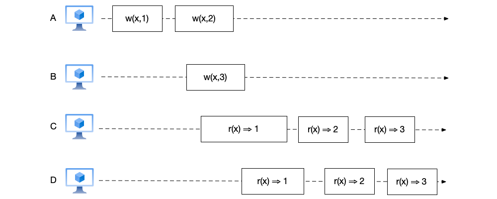
• As shown below, compared with the previous figure, the orders of node C and node D become $(r(x) \Rightarrow 3, r(x) \Rightarrow 1, r(x) \Rightarrow 2)$. This seems a bit counterintuitive. After all, the $w(x,1)$ operation on node A completes before the $w(x,3)$ operation on node B. However, the data read on nodes C and D is not in this order. But upon careful consideration, this ordering also does not violate the requirements of sequential consistency, because this read order both preserves the event order on the nodes and is globally consistent.

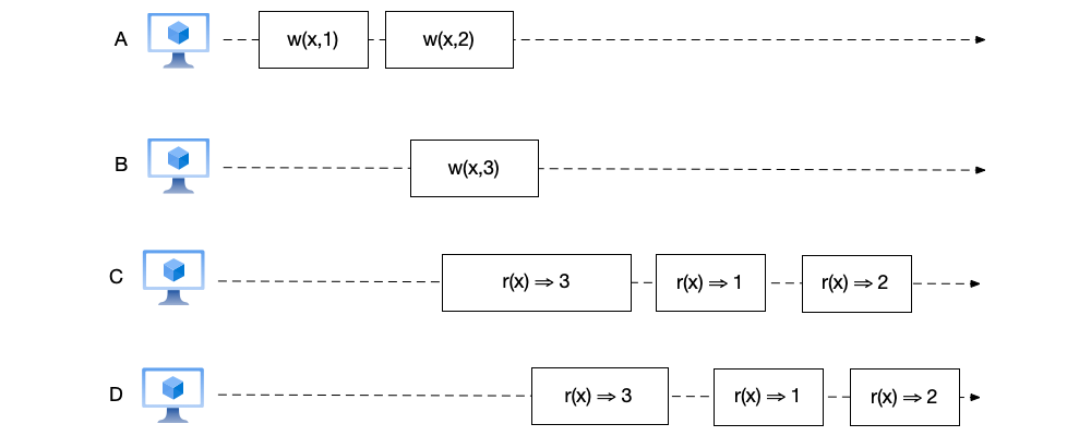
• As shown below, the orders of node C and node D are inconsistent, so this is not sequential consistency.

Among the above examples, the most counterintuitive and difficult to understand is the second example. However, this example reveals a characteristic of sequential consistency: sequential consistency does not require real-time occurrence of events. This can lead to situations where events ordered under a global clock are reversed under sequential consistency. For example, in the figure, $w(x,1)$ completes before $w(x,3)$, but under sequential consistency, the value of $x=3$ can be read first.

If the system design requires real-time guarantees for data consistency, then linearizability, which will be introduced next, should be chosen.

---

In many scenarios, the system only requires guaranteeing order, and the real-time requirement is not high. Such scenarios are suitable for implementing sequential consistency, for example:

• An account posts two tweets on a social platform. Synchronizing the tweets to different followers’ accounts may be delayed. Some followers’ accounts may only see the first tweet, while others may have already seen both. However, as long as the tweets are not out of order and are displayed on the timeline in the order they were posted by the account, it is acceptable.
• Some games with low real-time requirements (such as chess and card games) require player actions to be synchronized to the client in order to avoid state inconsistency.

Linearizability #

Next, we look at linearizability [9], sometimes also called atomic consistency [10] or strong consistency. It is currently the strongest consistency model among common consistency implementations.

Linearizability adds one condition on top of sequential consistency:

For events on different nodes, if they are not concurrent events (rectangles that do not overlap on the timeline), their execution order must also remain consistent after reordering.

That is, if the times of two events $a$ and $b$ satisfy $t(a) < t(b)$, event $b$ must see the result of event $a$’s operation.

Sequential consistency’s ordering requirements satisfy program order, while linearizability’s ordering requirements satisfy real-time, and the real-time requirement is stronger than program order. For example, for sequentially executed events on the same node, the event times definitely have a precedence order. For events with a causal relationship, their event times also have a precedence order.

This is the stronger data real-time requirement of linearizability compared to sequential consistency. With the guarantee of real-time, a system that provides linearizability can provide the illusion of having only a single copy.

Because linearizability has one more condition than sequential consistency, a system that satisfies linearizability naturally satisfies sequential consistency. The converse is not true.

---

Let us look at an example that satisfies sequential consistency but does not satisfy linearizability:

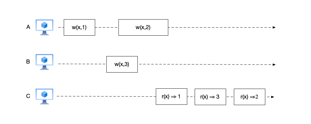
In the figure above, node C successively reads the three values 1, 3, and 2. To satisfy this order, the event ordering in the figure can only be: $(w(x,1), r(x) \Rightarrow 1, w(x,3), r(x) \Rightarrow 3, w(x,2), r(x) \Rightarrow 2)$.

We can see that this ordering satisfies the requirements of sequential consistency:

• Multiple events occurred on both node A and node B. The reordered event ordering preserves the event order on both nodes.
• No event rollback occurred. None of the three read operations read an older value.

However, this ordering does not satisfy the requirements of linearizability: node B’s $w(x,3)$ event occurs before node C’s $r(x) \Rightarrow 1$ event and does not overlap with it. However, in the ordering, $r(x) \Rightarrow 1$ is placed before the event $w(x,3)$.

---

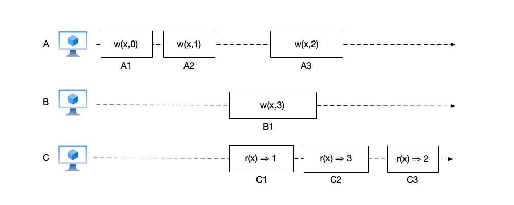
Let us look at an example that satisfies linearizability. As shown below, the event order of node C is $(r(x) \Rightarrow 1, r(x) \Rightarrow 3, r(x) \Rightarrow 2)$. For the convenience of explanation, the event names are labeled below these events:

• This order satisfies the event ordering on node A: first reading data 1, then reading data 2.
• Event C1 occurs after event A2 and overlaps with events A3 and B1. Therefore, it is reasonable for event C1 to read any of the values written by these three write events. However, if event C1 reads the result $x=0$ of event A1, it violates linearizability.
• Similarly, event C2 overlaps with events B1 and A3. It is reasonable for it to read 1, 3, or 2.
• Event C3 occurs after the last write event A3. Therefore, C3 must read $x=3$ written by A3.

---

Both sequential consistency and linearizability attempt to provide the illusion of “a single copy.” However, sequential consistency’s copy has no real-time requirement. For some scenarios with real-time requirements for data, only linearizability can be used. As shown below, we will see how distributed consensus algorithms implement linearizability.

• Two clients first request two nodes to query the current remaining number of tickets. Both return 1.
• Client A initiates a ticket purchase request to node 1. Node 1 decrements the remaining number of tickets by one. This operation is also replicated to node 2.
• Before the replication request reaches node 2, client B also initiates a ticket purchase request. Since the remaining number of tickets on node 2 is still 1 at this time, the purchase is successful, and the ticket is oversold.

---

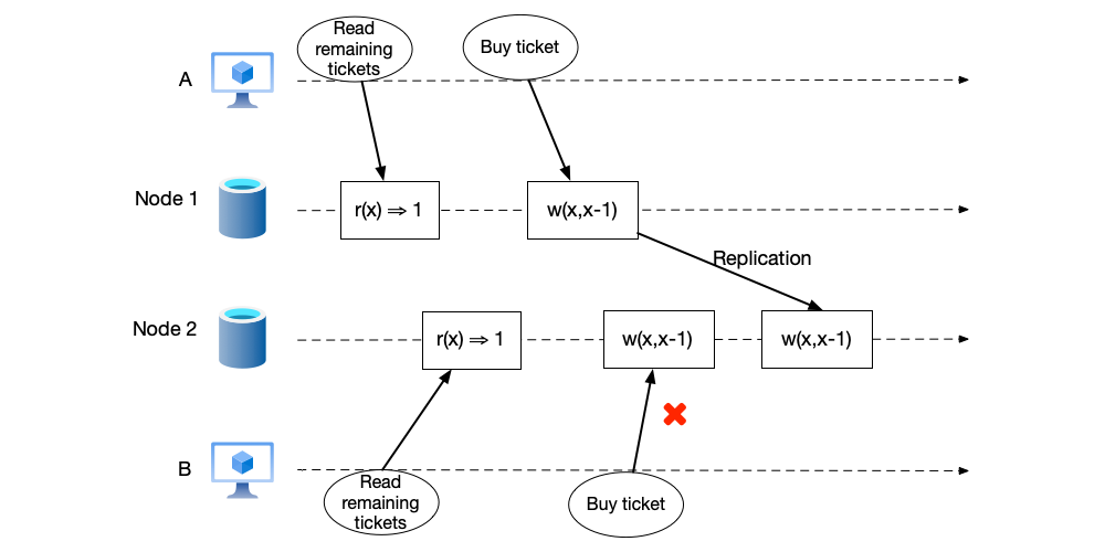
Note: Even if the system in the figure above satisfies linearizability, because there is a delay between client B’s two read and write operations, for such operations that first read and then modify based on the read value, a better approach is to use a CAS (compare and swap) operation: modifications are only made when certain conditions at the time of reading are met.

Causal Consistency #

Sequential consistency and linearizability are both strong consistency models. These two consistencies require that all replicas in the system can only have one order, which comes at a high cost in implementation. In many scenarios, such a strong consistency requirement is not needed. Causal consistency is a relatively weaker consistency guarantee. In this consistency model, only events with a causal relationship are required to maintain their order.

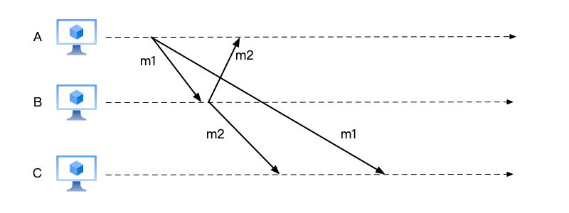
As shown below, A asks two other people the question (message m1) “Where shall we go to play today?” B replies (message m2) “Go to the movies.” If these two messages appear to user C in the order m2 before m1, the causal order is violated.

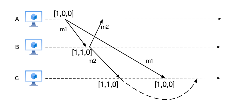
The vector clock introduced earlier can be used to guarantee causal order, as shown below:

• When A sends message m1, it carries the local vector clock [1,0,0].
• When B receives message m1 and sends message m2, it carries the local vector clock [1,1,0].
• After C first receives message m2, it finds that its vector clock is [1,1,0]. It will delay delivering this message until after receiving message m1.

---

One major problem with this causal order implemented using vector clocks is that the size of the vector clock is related to the number of nodes. In many cases, this can cause a large amount of data to be synchronized. In addition, there is another drawback: in some scenarios, it is impossible to know how many nodes are participating in the communication, and thus it is impossible to determine the array size of the vector clock.

For these situations, a custom logical clock can be designed for such scenarios that only need to guarantee causal order:

• Each user maintains an incrementing numeric ID. It is incremented each time a message is sent to the outside.
• When sending a message to the outside, the node’s ID and the message ID must be carried. If the message is a reply to another message, the parent message’s message ID must be carried.

With the message ID, the message delivery process is modified to:

• If the message has no parent message ID, it means it is not a reply to another message, and the message can be delivered directly.
• Otherwise, the message can only be delivered after the parent message has been delivered.

One question here is: how to determine whether the parent message has been delivered? The following approach can be used:

• Within each node, maintain a maximum numeric ID keyed by node ID, saving the maximum ID currently seen from another node.
• When the received parent message ID is not empty, extract the node ID and message ID from the parent message ID:
  • If the current maximum numeric ID for that node exists, take the currently saved maximum numeric ID. If it is greater than the message’s ID, it is considered delivered. Otherwise, it is not delivered. Messages whose parent messages have not been delivered need to be temporarily stored in the message queue to wait for delivery.
  • Otherwise, if the maximum numeric ID for that node has not been saved before, this definitely means the parent message has not been delivered.
• When a message is received, if there is no parent message ID, extract the node ID and message ID from the message, and update the maximum numeric ID corresponding to the node ID. Then, check the message queue based on the node ID and message ID to determine whether there are messages waiting for this message to complete delivery. If so, delete the message from the message queue to complete delivery.

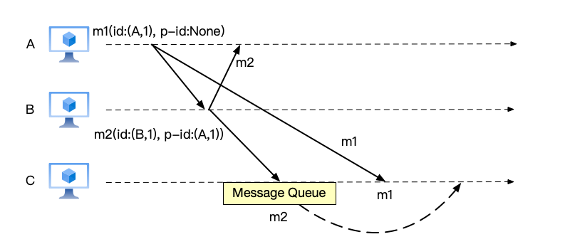
According to the above idea, let us re-implement the previous problem. As shown below, the id in the figure represents the message id, and p-id represents the parent message id. When there is no parent message id, p-id is None. The message id consists of a tuple of (node id, message id):

• When A sends message m1, the id information carried is (id:(A,1), p-id:None), indicating that it is a message sent from node A, the message ID is 1, and there is no corresponding parent message. That is, it is not a comment on another message.
• When B replies to message m2, the id information carried is (id:(B,1), p-id:(A,1)), indicating that it is a message sent from node B, the message ID is 1, and the parent message ID of this message is (A,1). That is, it is a comment on user A’s message with message ID 1.
• When C receives message m2, it extracts the parent message ID information, determines that the parent message has not completed delivery, and temporarily stores it in the message queue.
• When C receives message m1, it extracts the message ID information. Because this message has no parent message ID, it can complete delivery directly. After delivery is complete, it checks the message queue and finds that there is a child message waiting for delivery. It deletes message m2 from the message queue to complete the delivery of message m2.

Note: The above methods of using vector clocks and parent message IDs to implement causal consistency are only one implementation idea. In essence, as long as the logical clock adopted can satisfy the clock conditions, causal consistency can be achieved. Developers design logical clocks that satisfy the clock conditions based on different business scenarios to implement causal consistency.

---

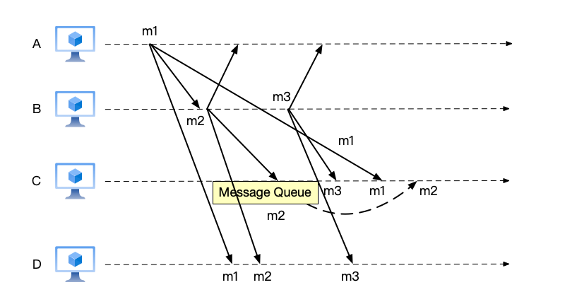
Systems requiring only causal consistency exhibit another characteristic: message out-of-order delivery is permitted as long as causal ordering is maintained and global consistency of messages across all nodes is not required. As shown below, node B sends message m2 and then sends message m3. Although node C first receives message m2, because message m2 needs to wait for m1 to complete delivery first, and message m3 has no parent message and can be delivered directly, the message delivery order on node C is (m3, m1, m2). The message delivery order on node D is (m1, m2, m3).

We can see that messages are allowed to be out of order here. For example, on node C, message m3 is delivered before message m2, which was sent by the same node. At the same time, the message orders on node C and node D are also inconsistent. Global consistency of message order across all nodes is not required.

This characteristic of causal consistency undoubtedly brings great convenience to implementation. Many scenarios with low consistency requirements can adopt causal consistency.

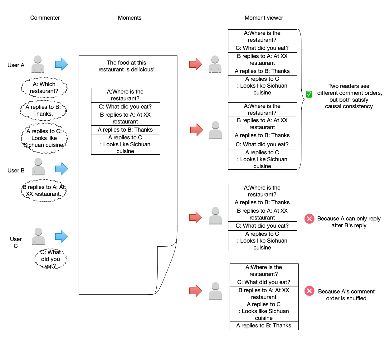
Let us re-examine the dynamic feed comment system design used at the beginning of this section to introduce consistency models. For this system, only causal consistency needs to be maintained. The figure below lists several possible comment orderings that people browsing comments may see. Although the top two are not the same, they both conform to the requirements of causal consistency because:

• The order of the three comments sent by the same user A is still maintained.
• The order of mutual comments between users (i.e., comments with a causal relationship) is still maintained.

However, the orderings in the bottom two arrangements do not meet the requirements. One violates the causal relationship by placing a reply to someone else’s comment before the comment itself. The other violates the order of the three comments sent by the same user A.

Eventual Consistency #

Finally, let us discuss eventual consistency, which was first proposed by Douglas B. Terry in [11] and later popularized by Werner Vogels [12, 13]. Although eventual consistency is often discussed together with the previous consistency models, strictly speaking, it is not a concept in the same category. To understand this, we must first understand the following two concepts: safety and liveness [14].

Safety and Liveness #

The definitions of safety and liveness first appeared in the paper [15]:

• Safety property: indicates that something bad will never happen.
• Liveness property: indicates that something good will eventually happen.

Safety is used to define properties that a system must absolutely not violate, for example, “data will never be lost,” “bank balance will never be negative,” “the system cannot have more than one leader node at the same time,” etc., all describe safety properties that the system needs to satisfy. Correspondingly, liveness defines certain properties that will eventually be guaranteed. These properties may not be satisfied at certain moments during system operation, but they will not be permanently violated. There will eventually be a moment when these properties are satisfied. For example, “requests will eventually be processed,” “expired data will eventually be cleaned up,” “multiple data replicas will eventually have consistent data,” all describe liveness properties that the system needs to satisfy.

It also needs to be emphasized here that:

• The properties described in safety are properties that the system absolutely cannot violate (the so-called “bad thing”), and they cannot be violated at any moment during system operation (the so-called “never happen”).
• The properties described in liveness are “good things” for the system. However, it is not required that the system must satisfy them at any moment. It is sufficient for them to be satisfied at a certain moment when events no longer change (the so-called “eventually happen”).

Eventual Consistency #

The core promise of eventual consistency is: if no new update operations occur, all replicas will eventually converge to the same state.

This description of eventual consistency fully conforms to the characteristics of liveness:

• It does not prohibit intermediate state inconsistency: it allows temporary “bad things,” such as reading dirty data.
• It guarantees that consistency will eventually be reached: “good things” will eventually happen.
• It cannot be judged as violated by a single observation: unlike safety, it does not require that the system never violates safety at any moment during operation.

Comparing eventual consistency with the strong consistency models introduced earlier:

• Strong consistency: Strong consistency requires that every read must be the latest value. Violating this condition is an error, so this is a safety requirement.
• Causal consistency: Causal consistency requires that events with a causal relationship must be satisfied in the system event arrangement at any moment. This is also a safety requirement.
• Eventual consistency: It only requires that consistency will be reached at some point in the future, without constraining the intermediate process. Therefore, this is a liveness requirement.

From this, we can see that eventual consistency is fundamentally different from the other consistency models discussed earlier. They are not discussing problems in the same category. Its core property is convergence, which means that all replicas in the system will eventually converge to the same value.

The liveness requirement of eventual consistency brings the following advantages and challenges to system design:

• Because it no longer requires the system to satisfy certain safety requirements at any moment, when system partitioning, network delays, and other problems occur, the system is allowed to have inconsistent replica data. This undoubtedly gives system designers greater flexibility. For example, developers can use asynchronous data replication to synchronize data among multiple replicas. When network partitioning problems occur, they can choose to lower the system’s consistency requirements and prioritize guaranteeing system availability.
• At the same time, for system users, they must also be prepared for the possibility of inconsistent data and implement data compensation measures. This shifts the complexity of handling inconsistent data to the users.

Typical application scenarios for eventual consistency include:

• DNS system: When a domain name updates its IP address, global DNS servers will not synchronize immediately. However, after a period of time (usually a few minutes to a few hours), all servers will reflect the latest IP address.
• Social media posts: After a user posts an update on social media, some of the user’s followers will not immediately see this update. However, after a period of time, they will also see the latest content.

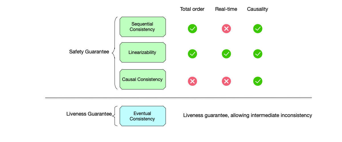
The figure below summarizes the consistency models explained in this section. In the figure, the safety-guaranteed models and the liveness-guaranteed eventual consistency model are strictly distinguished. Therefore, global ordering, real-time, and causality, which are safety guarantees, are not listed under eventual consistency. Eventual consistency allows inconsistent states to occur in the intermediate process.

CAP Theorem #

So far, we have discussed in detail a series of consistency models, from the strictest linearizability to the flexible eventual consistency. You can see that consistency models are like a ruler, precisely measuring the distributed system’s promise of data “freshness.” A natural question arises in our minds: since linearizability (strong consistency) is so intuitive and can greatly simplify application-layer logic, why don’t we always choose it? Why do systems like DynamoDB and Cassandra instead choose what seems to be an “unreliable” eventual consistency?

Imagine that to maintain linearizability, every node in the cluster must act like a disciplined army. Any data write must be confirmed by the “headquarters” (or rather, the majority of nodes) before it can take effect. This process works well when the network is calm.

But what if a network failure occurs—for example, the submarine cable between two data centers is bitten through by a shark—and our “army” is split into two isolated islands that cannot communicate? At this time, a “soldier” (node) stationed on an island receives a new write command. What should it do?

• If it insists on contacting the “headquarters” to guarantee consistency, then until the network recovers, it can only refuse service, and the system becomes unavailable.
• If it guarantees availability by arbitrarily accepting this command, then its data will diverge from the other half of the “army,” and consistency is broken.

From the above example, we can see that in the face of the harsh reality of “network partitioning,” the system is forced to face a dilemma. This fundamental and unavoidable trade-off is revealed by the CAP theorem, one of the most important cornerstones of the distributed field.

Next, let us deeply understand the CAP theorem, the “iron triangle” rule that governs all distributed system design. It will perfectly answer our question just now: why different systems choose to embark on different consistency paths.

The CAP theorem [16] is a conjecture proposed by Professor Eric Brewer of the University of California, Berkeley, in July 2000 [17]. Two years later, Seth Gilbert and Nancy Lynch proved the CAP conjecture theoretically [18], formally making it an important theorem in the field of distributed systems.

The CAP theorem states that for a distributed computing system, it is impossible to simultaneously satisfy the following three guarantees:

• C (Consistency)
• A (Availability)
• P (Partition tolerance)

For this reason, when designing a system, a choice must be made among these three guarantees. To truly understand this theorem, we must precisely define the specific meanings of these three guarantees.

Consistency

The consistency in the CAP theorem is linearizability. That is, after an update operation succeeds, the data on all nodes is completely consistent. This is a very strong constraint. The consistency mentioned in the BASE theorem introduced later is eventual consistency. This is the biggest difference between the two theorems.

Linearizability requires that once a write operation returns successfully, all subsequent read requests (no matter which node they are sent to) must be able to see this new data. The system behaves externally like a single-node system, where all operations are queued and executed sequentially. For example, on social media, after changing a username and clicking “save,” if you immediately refresh the page, what you see must be the new username. If you see the old one, strong consistency is not satisfied.

Availability

Availability requires that for any request sent to a non-failing node, the system can always return a non-error response within a finite amount of time. As long as there are still nodes alive in the cluster, it must be able to respond to requests. It cannot refuse service, nor can it wait indefinitely. Note that availability only guarantees “there is a response,” but does not guarantee that the response data is the latest.

For example, when visiting an e-commerce website, even if a few servers in the backend are down, the website can still be opened, and users can still browse products. The product inventory may not be the latest, but the website is “available.”

Partition Tolerance

Partition tolerance is the key and premise for understanding the CAP theorem. It requires that the system can continue to operate even when network connections between nodes fail (messages are lost or delayed), causing the cluster to split into multiple “network partitions” that cannot communicate with each other.

In distributed systems, the network is unreliable. Network cables between servers may be unplugged, and switches may fail. Partition tolerance means that we must design a system that can still work under these realistic conditions. As long as we choose to build a distributed system, we must assume that the network will have problems. We cannot choose “no partition tolerance.” Therefore, in modern distributed system design, partition tolerance is a fact, not an option.

Since partition tolerance is a property that the system must satisfy, when a network partition actually occurs, the system faces a fundamental trade-off: prioritize availability or guarantee consistency?

Let us use a classic bank transfer example to illustrate this process:

• A user’s bank account data, for high availability, is simultaneously stored on nodes N1 and N2 in two data centers.
• The initial balance is 1000.
• Now, the network connection between N1 and N2 is broken (a “network partition” has occurred), and they cannot communicate with each other.

At this point, an update request (withdraw 100) arrives at node N1. What should N1 do? There are two choices at this point:

Choice 1: Guarantee consistency (C), sacrifice availability (A) → CP system

To guarantee strong consistency, N1 must synchronize this withdrawal operation with N2. But now the network is broken, and N1 cannot contact N2. If N1 unilaterally changes the balance to 900, then the data on N1 and N2 will be inconsistent, which violates consistency. To guarantee consistency, N1 chooses to sacrifice availability, rejecting this withdrawal request or returning an error. But for the user who initiated the request to N1, the system is unavailable.

This is a typical CP system: it would rather not work than return a possibly incorrect piece of data.

Choice 2: Guarantee availability (A), sacrifice consistency (C) → AP system

To prioritize availability, N1 must respond to the user’s request. Although N1 cannot contact N2, it cannot let the user fail to withdraw money. The approach at this time is to accept this withdrawal request and change the local balance from 1000 to 900. At the same time, it will record this operation and find a way to synchronize it with N2 after the network recovers. At this point, the system is available to the user. However, before the network recovers, N1’s balance is 900, while N2’s balance is still 1000. The system is in an inconsistent state.

This is a typical AP system: it will try its best to serve, but the data seen by the user may not be the latest. It will synchronize the data later. This later synchronization mode satisfies eventual consistency.

The above is an introduction to the CAP theorem. However, in practice, systems operate over asynchronous networks where communication delays have no upper bound. Consequently, treating network partitions as a binary state is an oversimplification. More often, what the system faces is a sudden jitter in message delay, such as: nodes are busy and fail to respond in time, the system’s network suddenly jitters, etc. In addition, trade-offs are a continuous spectrum, not a binary switch. Real-world systems are not purely CP or AP. Many systems allow you to adjust the consistency level to different degrees, for example, by providing various compromise models such as “session consistency” and “read-your-writes consistency.”

Professor Eric Brewer also realized that in the earliest description of CAP theory, the impact of latency was not considered. In the paper published in 2012 [19], he added a description of latency:

In its classic interpretation, the CAP theorem ignores latency, although in practice, latency and partitions are deeply related. Operationally, the essence of CAP takes place during a timeout, a period when the program must make a fundamental decision—the partition decision:

• cancel the operation and thus decrease availability.
• proceed with the operation and thus risk inconsistency.

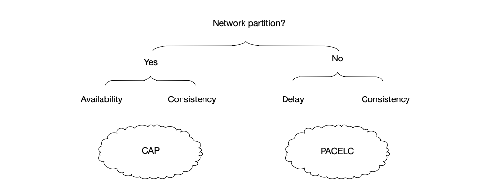
In 2010, PACELC proposed by Daniel J. Abadi of Yale University [20] can be seen as a supplement to the CAP theorem in terms of latency:

• If a network partition occurs, the system should make a choice between consistency and availability, just like the CAP theorem.
• Otherwise, system design should make a choice between latency and consistency.

Shortcomings and Insights of the CAP Theorem

The original CAP theorem had many problems, for example:

• The CAP theorem did not consider the impact of network latency. If the system is to maintain consistency, there is a time cost to synchronize data between the system’s nodes.
• The CAP theorem’s assertion that only two of the three properties can be chosen is also somewhat misleading. If there is no partition in the system, there is no reason to make a choice between consistency and availability. Secondly, this statement is too black and white, ignoring the fact that system operation is a spectrum. For example, the availability metric is a dynamically changing percentage. Consistency also has various levels of strength. Latency also has different time ranges in different application scenarios. Within these spectra, developers can customize the required characteristic parameters based on business scenarios.

In addition to the PACELC mentioned earlier, which extended the CAP theorem in terms of latency, Martin Kleppmann also discussed some shortcomings of the CAP theorem in [21].

Nevertheless, the purpose of proposing the CAP theorem was to guide system designers to think about whether a system should prioritize consistency or availability during design:

• AP (abandoning consistency): This means that when a network partition occurs, inconsistent data between the system’s nodes is allowed.
• CP (abandoning availability): This means that when a network partition occurs, in order to maintain consistency between the system’s nodes, the time to synchronize information is prolonged, which affects system availability.

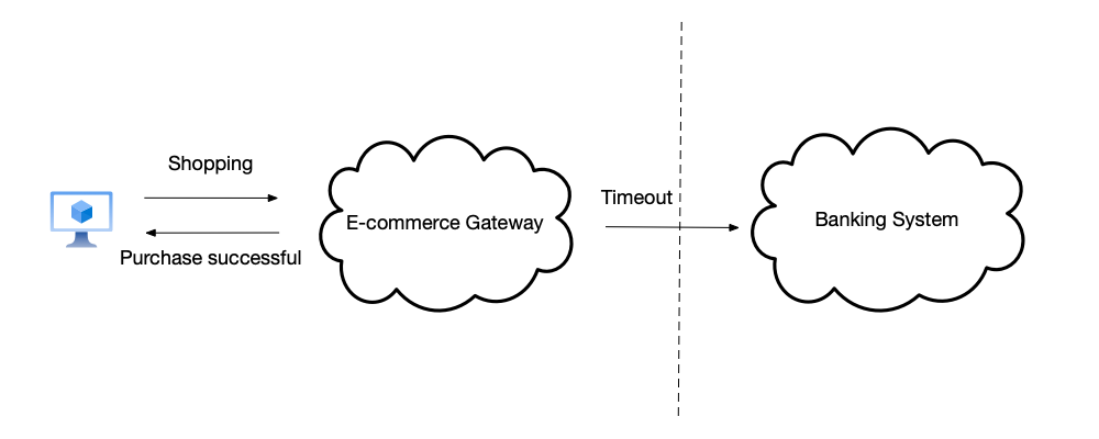
As shown below, when a user initiates a purchase request to an e-commerce platform, the e-commerce platform gateway and the bank system are located in different network partitions. When the deduction request initiated by the e-commerce platform to the bank system times out, it cannot respond to the customer that the purchase was successful. That is to say, in this business scenario, consistency should be prioritized over availability.

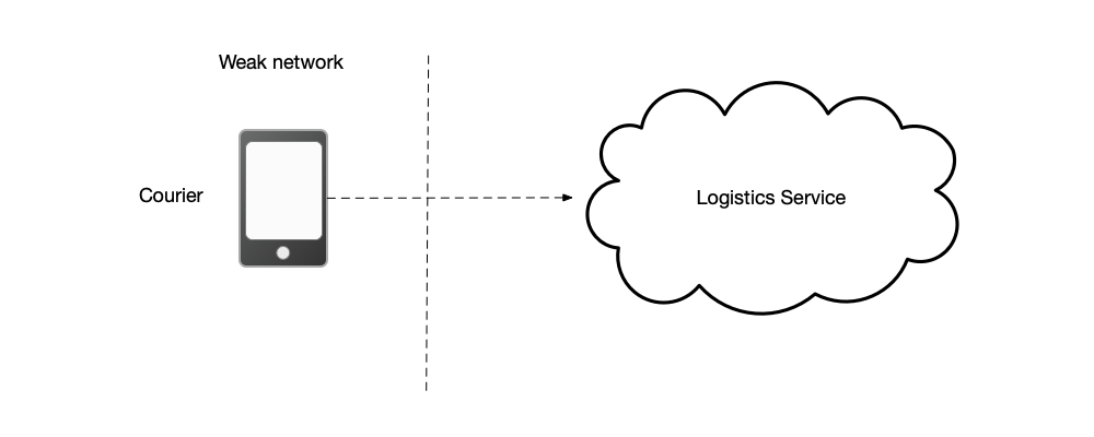
As shown below, when a courier picks up a package, in a poor network environment, the backend logistics platform cannot be reached. This can be considered as two network partitions being formed. In this case, availability is prioritized. The pickup data can be temporarily stored on the device, and the pickup is considered successful. When the network recovers, the data is synchronized to the logistics service.

The above are examples of making a choice between consistency and availability in the case of network partitioning. When there is no network partitioning, a choice must be made between service latency and consistency. As shown below, user A posts a new message on a social platform. This message needs to be synchronized to three different nodes. User B follows user A on the social platform, but when his request reaches node 3, user A’s message has not yet been synchronized to this node. In this scenario, nodes are allowed to return old data to the client to prioritize service availability.

Client-Centric Consistency Models #

Previously, we introduced several of the most common consistency models. When a system can only satisfy eventual consistency, the client may read stale, expired data. Nevertheless, the client still needs to satisfy some specific consistency requirements within a system that only provides eventual consistency to guarantee the client’s business. These consistency guarantees provided by the client are called “client-centric consistency models.” This section will introduce several common client-centric consistency models, which come from the paper [22]. The authors use a baseball game as an example to illustrate the usage scenarios of these client-centric consistency models. At the end of this section, this example will also be used as a summary.

Consistent Prefix #

Consistent Prefix ensures that the data read by the client is an ordered, continuous subset (prefix) of all write operations in the system. In other words, the data seen by the client reflects all write operations up to a certain point in time, and these operations are presented in the order they were written, without disorder or partial updates. The write order seen by the read operation is a logically consistent prefix. That is, data versions evolve in a certain order, and causal confusion does not occur, such as “seeing the result before the cause.”

As shown below, consider a scenario in a group chat of three people. User A asks: “Where shall we go to play today?” User B replies: “Go camping.” Then, from the perspective of the third person in the group, user C, even if message reception may be delayed, the above two messages should be guaranteed to arrive in order. This is what consistent prefix aims to guarantee.

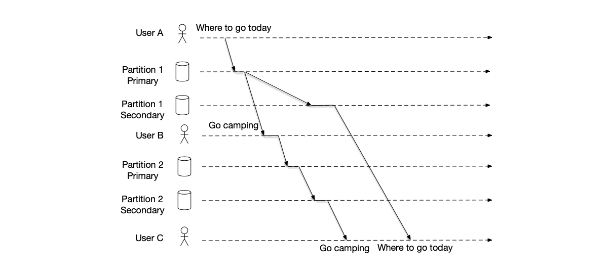
The key characteristics of consistent prefix are:

• Ordering: The data read reflects the actual order of write operations. For example, if the write operations are sequentially $\{W1, W2, W3\}$, the figure below shows several legal and illegal prefixes. Under the consistent prefix model:
  • The client may only read $\{W1\}$, or read $\{W1, W2\}$. Both of these cases conform to the consistent prefix requirement.
  • However, it will not read $\{W3\}$ (skipping W1 and W2 that occurred before W3), or $\{W1, W3\}$ (skipping W2), because neither of these cases is a legal prefix of the set $\{W1, W2, W3\}$.
• Prefix: The read result is a prefix of the write history, not a random or incomplete fragment. Still using the above example, $\{W1\}$ and $\{W1, W2\}$ are prefixes of $\{W1, W2, W3\}$, but $\{W3\}$ and $\{W1, W3\}$ are not.
• No partial writes: It does not return results of only partially completed write operations, ensuring data integrity.
• Weak consistency: Consistent prefix has lower requirements than strong consistency. It may not reflect the latest writes, but it guarantees that what is seen is a consistent “historical” fragment.

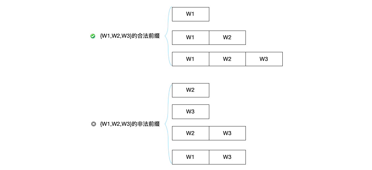
Consistent prefix is mainly used in the following scenarios:

• When reading multiple data objects, ensure that they come from the state of the same logical point in time (avoiding seeing partially updated inconsistent combinations).
• When write operations are progressive updates (rather than complete overwrites), guarantee that the intermediate state read is logically coherent. The client can read an ordered write history: the data version read must constitute a complete, logically continuous “historical fragment,” without skipping intermediate writes.
• In event-driven architectures, consistent prefix ensures that the event stream read by consumers is committed in order, such as in message queue systems.
• When replicating data in primary-backup multi-replicas, the backup node may lag behind the primary node, but consistent prefix guarantees that the data returned by the backup node is a complete prefix of the primary node’s writes.

A few examples:

• When reading multiple related data objects, if there is a dependency relationship between multiple pieces of data (such as orders and payment records), consistent prefix ensures that contradictory combinations are not read. For example, in an e-commerce payment scenario, seeing a payment record but not the corresponding order record.
• When reading incrementally updated data, if the writes are progressive updates rather than overwrite writes, consistent prefix ensures that these incremental change records can be read in order. For example, a bank account has two balance changes, from an initial balance of 0, first becoming a balance of 100, and then becoming a balance of 200. Consistent prefix should guarantee that these two change records can be read in order.

Monotonic Reads #

As shown below, user A’s comments need to be synchronized to two backup nodes. User B’s two read operations land on two different backup nodes, resulting in reading data the first time but not the second time. It looks as if time has “flowed backward.”

Monotonic Reads guarantees that during a client’s session, read operations will not experience time flowing backward. Under this model, the client may read old data, but it can guarantee that during the same session, the data read by the client will become newer and newer over time. Data rollback will absolutely not occur. For example, if the same client initiates two read operations on the same object in succession, the monotonic reads model guarantees that the value returned by the second read operation is either the same as the first or a more recently written value. Because of this characteristic, monotonic reads are also called “session guarantees.”

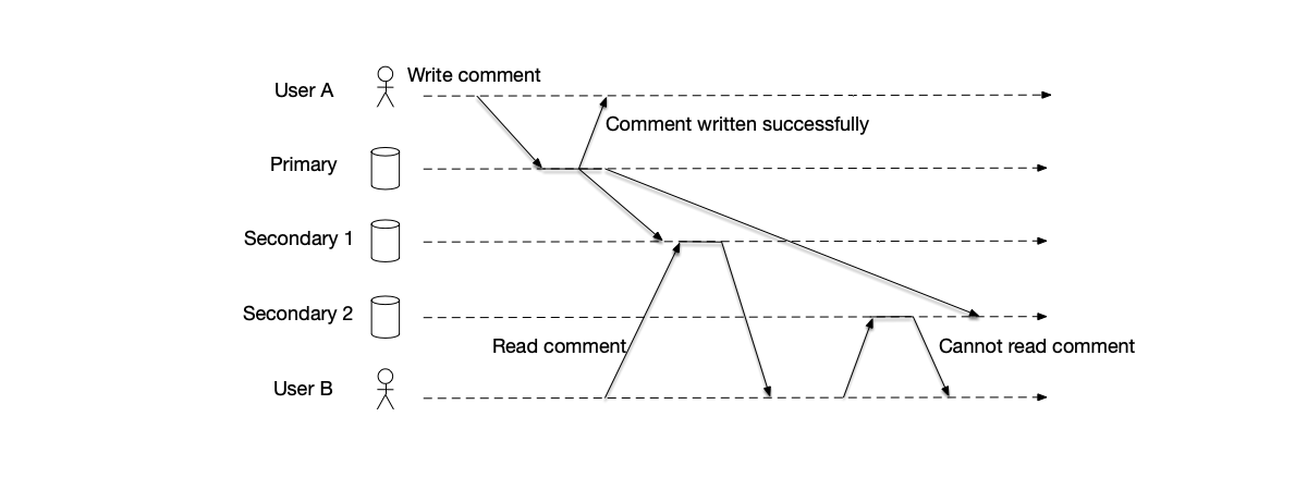
We can see that the two key characteristics of monotonic reads are:

• Preventing “time flowing backward”: Data rollback will not be seen across multiple requests.
• Not guaranteeing globally latest: Monotonic reads may read stale data, but still maintain monotonic increase.

It is important to note the difference between monotonic reads and consistent prefix mentioned above. Still taking the event set $\{W1, W2, W3\}$ as an example, monotonic reads allow reading an event set such as $\{W2, W3\}$, because after reading event W2, W3 is read, and the event has not rolled back. However, in consistent prefix, $\{W2, W3\}$ is not allowed, because this is not a legal prefix of the event set $\{W1, W2, W3\}$.

Common solutions for implementing monotonic reads include:

1. Session stickiness: The same client always reads data from the same replica. For example, requests can be routed through a session ID (such as Nginx’s ip_hash), or the client’s most recent read position can be recorded in the database proxy layer.
2. The client records the latest version number it has read, and subsequent requests require the server to return data greater than that version.

Read Your Writes #

As shown below, user A updates his profile on social media. The data returns a successful profile update after being successfully replicated to the primary node, and then it is synchronized to two backup nodes. If before the data has been synchronized to the backup nodes, user A tries to read the new profile, and the request is routed to a backup node that has not yet completed data synchronization, old data will be read. This will cause the user to mistakenly believe that the updated data has been lost.

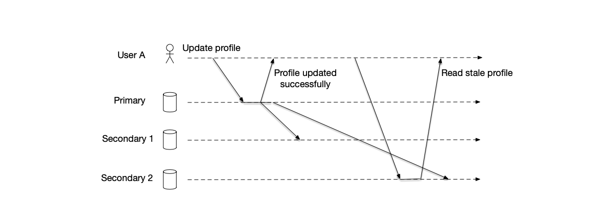
“Read your writes” ensures that the effects of all write operations by a client are visible to that client’s subsequent reads. In other words:

• If a client writes a new value to a data object and then immediately reads that object, the read operation will return the last value written by that client.
• If the client has no write operations, the behavior degrades to eventual consistency, and old values may be read.

Typical application scenarios for read your writes include:

• Social networks: After a user posts an update, his own page must be able to immediately see the content just posted, avoiding the situation of “post successful but cannot refresh it.”
• E-commerce: The order list must immediately display new orders to prevent users from repeatedly purchasing products.

The read-your-writes model can ensure that users can immediately see their changes after performing operations. If system design does not consider this, it may lead to problems such as “I changed my profile, why is it still showing the old one?” which affects user experience.

Common solutions for implementing read your writes include:

1. After the client successfully writes data, it records the current timestamp. When requesting to read data, it carries the timestamp of the most recent data write. The server guarantees to return data no earlier than that timestamp.
2. Based on certain parameters from the client’s write request, ensure that the client’s requests are always routed to replicas that have synchronized the write.

Baseball Game Example #

To explain the practical application of these client-centric consistency models in real business, the paper [22] uses a baseball game as an example to illustrate the data consistency problems faced by several types of people who need to read the current score. Assume that the game score is stored in a key-value store, and the scores of the visiting team and the home team are written to different storage keys.

The following gives a simplified baseball game flow, with some simple explanations:

• The two sides of the game are the home team and the visiting team, with an initial score of 0.
• The game is divided into 9 innings. In each inning, the visiting team and the home team take turns as the batting side and the defending side. The batting side hits the ball with a bat and then runs the bases, successively stepping on first base, second base, third base, and returning to home base to score 1 point. The defending side prevents the opponent from scoring by pitching, catching, and throwing out, and strives to get 3 batters out before switching offense and defense.

Based on the above baseball game flow, the code flow for updating the score is as shown below.

Write ("visitors", 0);
Write ("home", 0);

for inning = 1 .. 9
    outs = 0;
    while outs < 3
        visiting player bats;
        for each run scored
            score = Read ("visitors");
            Write ("visitors", score + 1);

    outs = 0;
    while outs < 3
        home player bats;
        for each run scored
            score = Read ("home");
            Write ("home", score + 1);
end game;

The table below simulates the scores and total score of each inning of a baseball game when it has progressed to the 7th inning. The visiting team has completed this inning, while the home team has not yet started. The total score is 2-5.

	1	2	3	4	5	6	7	8	9	Total
Visitors	0	0	1	0	1	0	0			2
Home	1	0	1	1	0	2				5

Based on the score sequence shown in the table above, the process sequence for updating the game score is as shown below.

Write("home", 1);
Write("visitors", 1);
Write("home", 2);
Write("home", 3);
Write("visitors", 2);
Write("home", 2);
Write("home", 3);

When the game has progressed to the 7th inning with a total score of 2 to 5, according to different consistency models, the following scores may be read:

• Strong consistency: Only the current latest score of 2-5 can be read.
• Eventual consistency model: Any score may be read, including situations where the score of a certain inning does not appear in order. For example, a score of 0-3 may be read. From the table, we can see that the game proceeds in order, and a score of 0-3 is absolutely impossible. Reading such a score only indicates that when reading the scores of the two teams at a certain time, the visiting team’s score read is older than the home team’s score read. In the eventual consistency model, the score eventually settles at 2-5.
• Consistent prefix: In consistent prefix, the score read satisfies the “alternating change” order of the visiting team and home team. That is, in any inning, the visiting team’s score is updated first, because the visiting team becomes the attacking side first, and then the home team’s score is updated. For example, after reading a score of 0-1, the next score read is 1-1, because the visiting team scored 1 point first in the third inning, and then it is 1-2, because the home team also scored 1 point in the third inning.
• Monotonic reads: In monotonic reads, regardless of whether the home team or visiting team score is read, there is no data rollback. Therefore, after reading 1-3, scores before this will no longer be read. Only scores after this score will be read.
• Read your writes: If it is the writer, strong consistency must be satisfied, so only the score of 2-5 can be read. Otherwise, for non-writers, the data read is the same as the set of scores that the eventual consistency model may read.

Consistency Model	Possible Scores Read
Strong Consistency	2-5
Eventual Consistency	0-0, 0-1, 0-2, 0-3, 0-4, 0-5, 1-0, 1-1, 1-2, 1-3, 1-4, 1-5, 2-0, 2-1, 2-2, 2-3, 2-4, 2-5
Consistent Prefix	0-0, 0-1, 1-1, 1-2, 1-3, 2-3, 2-4, 2-5
Monotonic Reads	After reading 1-3: 1-3, 1-4, 1-5, 2-3, 2-4, 2-5
Read Your Writes	For the writer: 2-5; for any other non-writer: the same set of scores as eventual consistency

After understanding the scores of each stage of this simulated baseball game and the possible scores under various consistency models, let us look at what consistency requirements different types of readers need to satisfy for such a game with real-time score updates. Although strong consistency can be used to satisfy all readers’ needs, we will see that in the baseball game example, by analyzing the consistency requirements of different types of readers, weaker-than-strong-consistency read guarantees can be used to satisfy the needs while gaining performance advantages. In this example, the readers of the baseball game score are divided into: official scorekeeper, umpire, radio reporter, sports reporter, statistician, and stat watcher.

---

Official Scorekeeper

The official scorekeeper is responsible for updating the game score, writing both sides’ scores to the key-value store in real time. The code below demonstrates the workflow of the official scorekeeper updating the visiting team’s score (the logic for updating the home team’s score is similar). The scorekeeper must increment the previous score by one. Therefore, before each new score update, the latest score must be readable. Otherwise, it may lead to incorrect score recording. For example, if the home team previously scored 5 points, then when getting the 6th point, if eventual consistency is used to read the score at this time, it may return any score between 0 and 5.

It can be seen that the scorekeeper needs strongly consistent data. However, in the baseball game scenario, because the scorekeeper is the only entity that changes the score, only the “read your writes” guarantee is needed. This will also achieve the effect of strongly consistent data reads. It can be seen that through analysis of specific scenarios, weaker consistency can be used to achieve business goals.

This subtle distinction greatly improves the scorekeeper’s read performance. If strong consistent reads are used, the system would have to assume that while the official scorekeeper is updating the score, another client is also updating the data. If this is the case, the system needs to access most servers to ensure that the data just read is the latest. When using read-your-writes consistency, the system only needs to remember which servers previously executed write operations, and it can read the data previously written by itself from these servers.

score = Read ("visitors");
Write ("visitors", score + 1);

Umpire

After the first half of the ninth inning of a baseball game, that is, after the visiting team has batted and before the home team is about to bat, a judgment is made as to whether the game can be terminated early. Since this is the last inning, if the home team is already leading in score, the remaining games do not need to be played, and the home team can be directly declared the winner. According to this rule, the umpire does not care about the game score for most of the game. Only after the first half of the ninth inning will the algorithm below be used to determine whether the game can be terminated early. Unlike the scorekeeper, the umpire never records the score, but only reads the values written by the official scorekeeper. Therefore, to receive the latest information, the umpire must use strong consistency to read data.

if first half of 9th inning complete then
    vScore = Read ("visitors");
    hScore = Read ("home");
    if vScore < hScore
        end game;

Radio Reporter

Radio stations regularly broadcast the real-time score of the ongoing game. Modern equivalents include sports applications that update the game score in real time while the game is in progress. The workflow of this type of reader is as shown below.

The real-time score broadcast during the game may not be the completely latest score. For example, after the score changes, while the radio station is reporting the latest score, the score changes again. Then the score just broadcast is not the current latest result. Therefore, when the data read cannot satisfy strong consistency, what form of eventual consistency is acceptable for this type of score broadcaster?

First, the reporter absolutely does not allow reading non-existent scores. A score of 0-3 is absolutely impossible during the game. Reading such a score only indicates that when reading the scores of the two teams at a certain time, the visiting team score read is from the second inning or earlier, while at the same time the home team score from the 4th inning is read. If such a score is read, it is unacceptable for the audience watching the score broadcast.

Therefore, the reporter requires that all his read operations be performed on a consistent prefix snapshot that includes the writes executed by the scorekeeper. This way, the reporter can read a score that existed at a certain point in time, without forcibly obtaining the current latest score.

However, merely satisfying consistent prefix during reads is not enough. For example, it cannot happen that the score read at a certain moment is 2-5, and then later a score of 1-3 is read, because the game score satisfies monotonic increase. Therefore, it is unacceptable for contradictory scores such as 2-5 and 1-3 to appear successively in the report.

Therefore, in addition to satisfying consistent prefix, the reporter’s data reads also need to guarantee monotonic reads.

do {
    vScore = Read ("visitors");
    hScore = Read ("home");
    report vScore and hScore;
} while (match is not end)

Statistician

The team statistician is responsible for tracking the statistics of the team and players in each game of the season. As shown below, after the game ends, the statistician reads the home team’s score and updates it into the statistics for the entire season. When the game ends, a strong consistent read of the final score of this game must be performed. Similarly, when reading the season’s cumulative score, a strong consistent read is also required. Otherwise, if expired data is read, omissions will occur when updating the season’s total score. However, considering that the team statistician is the only entity that executes writes to the database for the season’s total score, the read-your-writes guarantee can also be used to update the season’s total score.

Wait for end of game;
score = Read ("home");
stat = Read ("season-runs");
Write ("season-runs", stat + score);

Stat Watcher

Other personnel who regularly check the team’s season statistics can generally accept eventual consistency. In the code below, it is assumed that these statistics are only updated once a day. Slightly outdated data is completely acceptable.

do {
    stat = Read ("season-runs");
    discuss stats with friends;
    sleep (1 day);
}

The table below summarizes the consistency models that each type of participant needs to satisfy. Here we can see that by utilizing specific scenario knowledge, weaker consistency reads can be used to achieve the effects required by different businesses without sacrificing consistency.

Participant	Consistency Model
Official Scorekeeper	Read Your Writes
Umpire	Strong Consistency
Radio Reporter	Consistent Prefix and Monotonic Reads
Statistician	Strong Consistency, Read Your Writes
Stat Watcher	Eventual Consistency

Leaderless Replication #

In the primary-backup replication mode introduced earlier, there is a primary node in the system. This is a centralized architecture: all write operations must pass through the unique “primary node” (Leader), and then be replicated by the primary node to the “backup nodes” (Follower).

The biggest problem with primary-backup replication is that the primary node itself is a single point of failure. If the primary node crashes, the entire system loses its write capability. Time must be spent on failover to elect a new primary node. During this election window, the system is unavailable.

In pursuit of extreme high availability and low latency, especially the availability of write operations, engineers designed another paradigm—leaderless replication. Its core philosophy is: all nodes in the system are equal, and any node can directly receive write requests.

Leaderless replication is another replication strategy in distributed systems. It gained prominence after Amazon’s 2007 paper [24] was published. In fact, such a replication strategy was already proposed earlier in [23]. Compared with the centralized architecture of primary node replication, the architecture design without a primary node is also called a “decentralized” architecture. Its ideas profoundly influenced the subsequent architectural design of Bitcoin. In Bitcoin’s architecture, any Bitcoin wallet is a node in this distributed system and can receive and process user requests.

---

Different from traditional primary-backup replication, the core characteristics of leaderless replication are:

• No central node: All replicas have equal status. There is no primary node responsible for coordinating write requests, so there is no primary-backup switch problem when the primary node fails in primary-backup replication.
• Client direct connection: The client needs to send read and write requests to multiple replicas simultaneously. Therefore, how to guarantee the arrival order of client requests becomes a thorny problem.
• Eventual consistency: Leaderless replication cannot provide the consistency guarantees in the previous consistency models. It can only achieve eventual consistency of data across multiple replicas through conflict resolution mechanisms (such as quorum, version vectors, etc.).

The advantage of leaderless replication is that because there is no central node and all replicas have equal status, it can tolerate node failures more easily than a centralized architecture. In primary-backup replication, the primary node becomes a single point of failure in the system. Once the primary node fails, the entire system cannot work normally. Other nodes need to be switched to the central node to continue service. In leaderless replication, as long as the number of nodes available for writing is satisfied, the system is still available. The data redundancy mechanism used in leaderless replication is the quorum mechanism.

Without a central node to serialize data writes, concurrent updates can easily lead to conflicts across multiple replicas. The client may read different data on different replicas, and the client needs to resolve the problem of inconsistent read data. At the same time, because the data on multiple replicas is not fully synchronized, mechanisms are also needed to guarantee eventual consistency of data between replicas.

This section will combine the Dynamo paper to explain the difficulties and solutions of leaderless replication.

Overview #

Amazon is one of the world’s largest e-commerce websites. It initially used relational databases to store business data. As the business expanded, the following patterns emerged in their storage service usage [24, 25]:

• The complex relational query functions of relational databases are not used much in business. Approximately 70% of operations are key-value type queries, i.e., only using the primary key to return a row of data, without complex multi-table queries (Join) in relational databases. Approximately 20% of operations will return multiple rows of data, but still only operate on a single table.
• Routing jitter, component failures, and network partitions are frequently faced situations. However, for e-commerce business, it is necessary to ensure that customer modification requests are successful in the vast majority of scenarios, i.e., satisfying “always writeable.” For example, users modifying items in their shopping cart is a common operation in an e-commerce business. If modification failures occur, it will affect user experience.

Taking the shopping cart as an example, the operation of a user adding an item to the shopping cart must absolutely not fail. If the user cannot add an item due to database partitioning, node downtime, and other issues, the user is likely to be lost. In comparison, briefly displaying a slightly outdated shopping cart (such as one lacking the item just added) is a much smaller loss. These business observations made Amazon’s engineers rethink the design of storage services suitable for their business. In traditional relational databases:

• The replication function of relational databases is very limited, and usually relies on sacrificing availability for consistency. This does not conform to the aforementioned situation where large e-commerce websites frequently face various failures.
• Most e-commerce services only use the primary key for retrieval and do not need the complex query and management functions provided by relational databases. These additional functions require expensive hardware and specialized skills, but the services do not actually use them. The end result is that using relational databases is very uneconomical.

This business need gave birth to Dynamo’s core design philosophy: sacrifice strong consistency in exchange for extreme high availability. This is the starting point for understanding all of Dynamo’s technologies.

Based on these considerations, Amazon designed the Dynamo system to replace relational databases. It only provides two interfaces for querying data based on the primary key: put(key, context, object) and get(key). The parameter context here stores metadata about the data, such as multiple versions of the data. We will see later how this information is used to resolve data conflicts.

The system makes the following assumptions about users:

• ACID: If ACID properties are to be satisfied, system availability will be sacrificed. The Dynamo system does not provide ACID properties. Instead, it provides eventual consistency, while also not providing any isolation guarantees.
• Efficiency: For Amazon’s services, system availability and latency are placed at the highest consideration in system design.

Overall, Dynamo has the following characteristics:

• Decentralised: Each node in the cluster assumes the same responsibilities and provides the same functions. The system is entirely peer-to-peer. There is no concept of leader or follower nodes.
• Highly Available: Dynamo distributes data across nodes and manages multiple replicas. Each node can handle read and write operations on data by forwarding requests to the nodes that store the data.
• Eventually Consistent: In order to provide an always-available and always-writeable data store, it sacrifices data consistency for availability. At a specific point in time, for a given data item, different replica nodes may disagree on the value of a key, but updates will eventually reach all replicas.
• Fault Tolerant: Data is distributed and replicated across multiple nodes to provide redundancy. A data subset only becomes unavailable when all replicas are unavailable. DynamoDB can be configured to replicate data to nodes located in different geographical data centers. This means that even if an entire data center fails, the cluster can remain available.
• Scalable: By adding or removing machines to the cluster, read and write throughput can be increased or decreased linearly. Dynamo can seamlessly handle data redistribution to adapt to such changes. Scaling the cluster requires no downtime, and operational overhead is minimal. Data redistribution also reduces the amount of data that a single node must store.

Read-Write Quorum Mechanism #

In leaderless replication, there is no “primary node” to uniformly issue commands. How does the system guarantee that data is eventually consistent? The answer is to borrow the “voting” mechanism from the real world, namely quorum, mentioned earlier. Let us see how this mechanism is used in leaderless replication to guarantee eventual consistency of data.

In the quorum mechanism, there are three key variables:

• N: Total number of replicas: a piece of data is replicated into N copies and stored on N different nodes.
• W: Write quorum: a write operation must be successfully written on W replicas before it is considered a “successful write.”
• R: Read quorum: a read operation must successfully read data from R replicas before it is considered a “successful read.”

In leaderless replication, because there is no primary node, it is necessary to initiate write operations to multiple replicas in the system simultaneously. That is, how many nodes’ responses must be received for read and write operations before the request is considered successfully processed? This depends on the parameter configuration in the quorum mechanism.

Let us start our discussion with the simplest system composed of 3 nodes. In such a distributed system, assume that the client only writes data successfully to one node and considers the write successful. Similarly, read requests also only read data from one node and consider the latest data to have been read. Since the system is composed of 3 nodes, this mechanism may read old data. As shown below, the client writes data to nodes A, B, and C at time t1. The write request sent to node B is lost for some reason. After the client receives the write request response from node A, it considers the write successful. When sending a read request to node B again, it reads the old value at time t0.

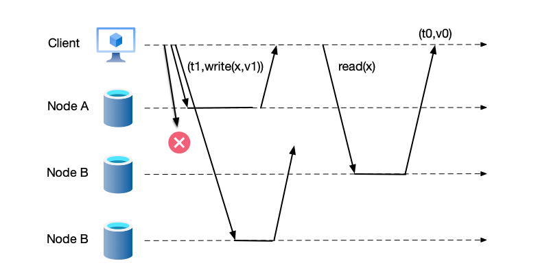
From the above example, it can be seen that in a system composed of 3 nodes, when writing to 1 node successfully is considered successful, reading data from only 1 node may read old data. The reason is: under this data configuration, the node where the write is successful may not overlap with the node where the read is performed. Only by guaranteeing that the sets of nodes for reading and writing overlap can it be guaranteed that at least one node in the read data stores the latest data. In this example of 3 nodes, the following read-write node quantity configurations can all satisfy the overlap condition:

• Writing to 2 nodes successfully is considered a successful write ($W=2$), and reading from 1 node ($R=1$) during reading.
• Or, writing to 1 node successfully is considered a successful write ($W=1$), but reading needs to be performed from 2 nodes ($R=2$), as shown below.

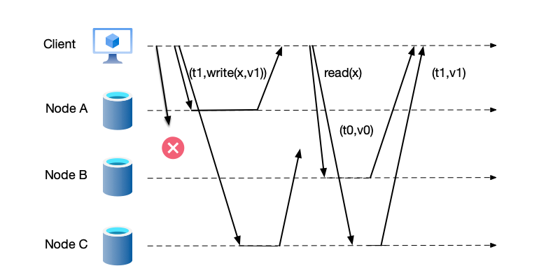
Generalizing the case of a 3-node system, if there are N nodes in the system, the set of replicas responding to write requests is called the write quorum, and the number of elements in this set is $w$. The set responding to read requests constitutes the read quorum, and the number of elements in this set is $r$. The quorum mechanism requires that the write quorum and the read quorum must have a non-empty intersection, i.e., satisfying $W + R > N$. According to the pigeonhole principle, this guarantees that read and write operations have at least one overlapping node, so the latest value can definitely be read in the read data.

The commonly used majority quorum in distributed systems is defined as a subset of more than half of the nodes, for example:

• In the 3-node system composed of A, B, and C, there are 4 majority quorums: $\{A,B\}$, $\{A,C\}$, $\{B,C\}$, and $\{A,B,C\}$.
• Generalizing, if the number of nodes in the system is odd, any set composed of more than $\lfloor \frac{n+1}{2} \rfloor$ nodes constitutes a majority, such as 2 out of 3, 3 out of 5. If the number of nodes in the system is even, any set composed of more than $\lceil \frac{n+1}{2} \rceil$ nodes constitutes a majority, such as 3 out of 4, 4 out of 6.

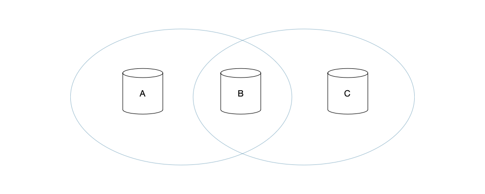
Dynamo adopts a consistency protocol similar to a quorum arbitration system, allowing users to flexibly configure the W and R parameters based on their business scenarios. The settings of W and R determine the system’s consistency level:

• Strong consistency: R, W, and the number of nodes N need to satisfy the relationship $R + W > N$. That is, at least one of R and W must exceed $N/2$. This guarantees that the replica sets of R and W operations definitely have an intersection.
• Eventual consistency: When $R+W \leq N$, the system only guarantees eventual consistency.

Referring to the discussion of data replication modes, the quorum read-write arbitration algorithm can be classified as a semi-synchronous replication mode. However, because this algorithm can be configured with different R and W parameters, under different configurations it can become different replication modes:

• $R=1, W=N$: At this point, the system is in fully asynchronous mode for read operations, while write operations become fully synchronous mode.
• $R=N, W=1$: At this point, the system is in fully synchronous mode for read operations, while write operations become fully asynchronous mode.
• $R=N, W=N$: At this point, the system is in fully synchronous mode for both read and write operations.

Data Conflict Problem #

The quorum mechanism solves the consistency problem of the same read and write data operation, but it does not solve the problem of inconsistent order that may occur when data is modified concurrently. In leaderless replication, because there is no primary node to coordinate write requests, any node can process write requests. Therefore, there is no guarantee of order between requests, and simultaneous concurrent write operations on the same data may occur. The arrival order of these requests at different nodes is inconsistent, leading to “write-write conflicts.” Different replicas may store different “latest values.”

As shown in the leaderless replication architecture below, two clients simultaneously modify the same data. The write request from client 1 to node B lags behind the write request from client 2 to node B, while for the other two nodes A and C, the request from client 1 arrives first. If not handled, conflicting data will appear on the nodes.

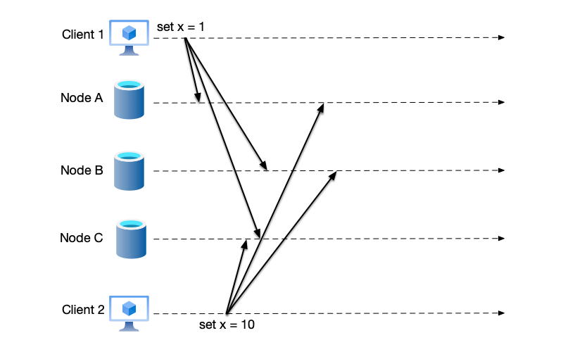
The simplest strategy for resolving concurrent write conflicts is last-write-wins (LWW). This strategy attaches a timestamp precise to microseconds or nanoseconds to each write. When a conflict occurs, the data with the newest timestamp wins. However, this strategy heavily relies on clock synchronization across all nodes. If the clock is inaccurate, it may lead to new data being overwritten by old data.

Let us look at how Dynamo resolves concurrent write conflicts. To address data conflicts, two fundamental questions must be answered: when to resolve the conflict, and who resolves it.

In traditional relational databases, conflicts are resolved when a data write request is received. This guarantees low read complexity because the data read by the client is conflict-free. However, in such systems, if most replicas cannot be accessed at any time, write requests will be rejected. Dynamo’s design is the opposite. Its goal is to achieve “always writable.” If client write requests are rejected when network partitioning or failures occur, it will result in a very poor user experience. This need led Dynamo to place the complexity of resolving data conflicts on read operations, to guarantee that write requests are never rejected.

After answering the question of when to resolve conflicts, let us look at who resolves data conflicts: the database or the application. If the database handles conflict resolution, only limited strategies are typically available, such as the aforementioned LWW mechanism. On the other hand, the application truly understands what the data describes. It can autonomously choose the conflict resolution method that is best for user experience. Taking the shopping cart application as an example, this type of application can implement a solution that “merges” multiple conflicting versions of data. In many cases, some application developers may not want to implement their own conflict resolution mechanism. In this case, the conflict resolution problem is delegated to the database, degenerating into choosing some simple strategies, such as using last-write-wins.

Dynamo chooses to have the application resolve conflicts when reading data. When the system cannot automatically resolve conflicts, it returns all conflicting versions (for example, two shopping carts with different contents) to the client application. The application-layer business logic decides how to “merge” these versions, and then writes the merged new version back to the system. Returning to the previous example of reading old shopping cart data, in Amazon’s application, similar data inconsistency is tolerable to guarantee availability. If the user then continues to modify from the old shopping cart data read out, it is equivalent to two branches of shopping cart data appearing. The system will retain each modification as an immutable version of the data. If multiple versions can be merged, they will be merged. Otherwise, all versions of the data will be returned to the client, and the application will resolve the data conflict.

Dynamo uses vector clocks to save multi-version data. If multi-version data can be determined to have a chronological order based on the vector clock algorithm, then data merging can be performed. Otherwise, all multi-version data that cannot be merged is returned to the application.

As shown below, vector clocks are used to represent different versions of the same data. The format is “[(node, counter)]”. The object has undergone the following modifications:

• The client’s first write data request is processed by node x. Since it is the first write, the system creates object D1, whose vector clock is [(x,1)].
• The client updates the data, and the request is sent to node x again for processing. Therefore, data object D2 is obtained, and its vector clock is [(x,2)]. According to the principle of vector clocks, object D2 is the descendant of object D1, so object D1 can be directly overwritten.
• The next two data modifications by different clients are no longer processed by node x, but are sent to nodes y and z respectively. Since these two modifications are the first data modifications on these two nodes respectively, two objects D3 and D4 are obtained. Both add their own node’s version number to the vector clock.
• Next, a client performs a data modification again. Two different versions of objects D3 and D4 are read from nodes y and z. Neither modification is reflected in the other’s modification, so data merging cannot be performed. Both versions must be retained. Finally, data D5 is written to node x.

In the above process, first, coverage merging is performed based on the causal relationship between versions (for example, D2 version data can overwrite D1). Data that cannot be merged (for example, D3 and D4 versions) will be retained simultaneously and returned to the client together. The client application-layer logic decides how to use these multi-version data.

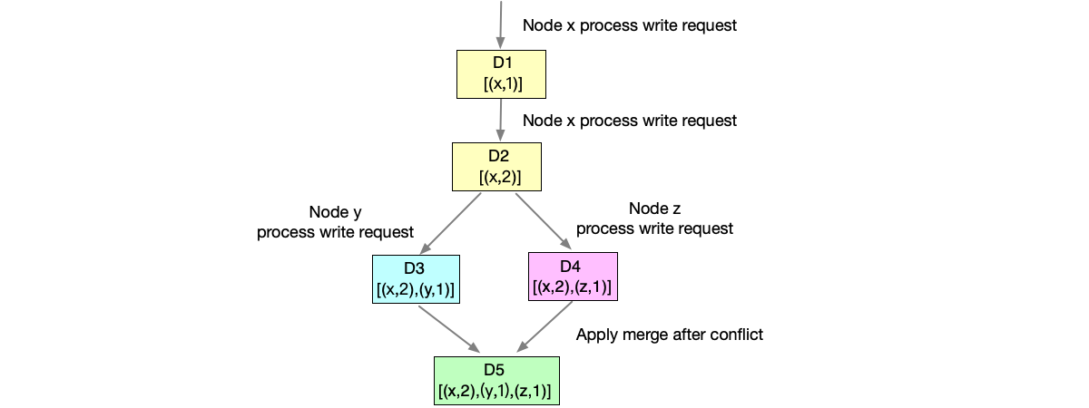
Cluster Membership Management #

In Dynamo, there is no “primary node” or other centralized coordination service. Therefore, the cluster must solve a fundamental problem itself: how does a node know about the existence and status of all other nodes, and which data is responsible for which nodes? The gossip protocol is the technical means Dynamo uses to solve this problem. It achieves decentralized cluster management by randomly propagating membership status information between nodes, effectively solving key problems such as node addition and removal, failure detection, and status synchronization. This mechanism enables Dynamo to maintain a consistent view of cluster members without a central coordination node, while possessing high availability and elastic scalability.

The gossip protocol is a probabilistic propagation-based distributed communication mechanism. Its core idea simulates the spread of epidemics in a population. Its main working principle is:

First, Dynamo solves the problem of new nodes joining the cluster through seed nodes. Seed nodes are pre-configured fixed nodes. All newly joined nodes first connect to seed nodes to obtain current cluster membership information. The existence of seed nodes ensures that new nodes can smoothly join the cluster, avoiding logical isolation problems. Even if some seed nodes fail, as long as at least one seed node is alive, new nodes can still join the cluster. This greatly improves the system’s fault tolerance.

Secondly, Dynamo uses vector clocks to record version information of membership status. Each node maintains a vector clock, where each element corresponds to a node’s counter, representing the number of times that node’s status has changed. When nodes exchange membership information, they also exchange their respective vector clocks. Through vector clock comparison, nodes can determine which membership information is the latest version and update the local status accordingly. This effectively resolves version conflicts in membership information synchronization.

As shown below, cluster nodes discover and track other nodes through the gossip protocol. As this process continues, eventually all nodes in the cluster can perceive the operating status of all other nodes.

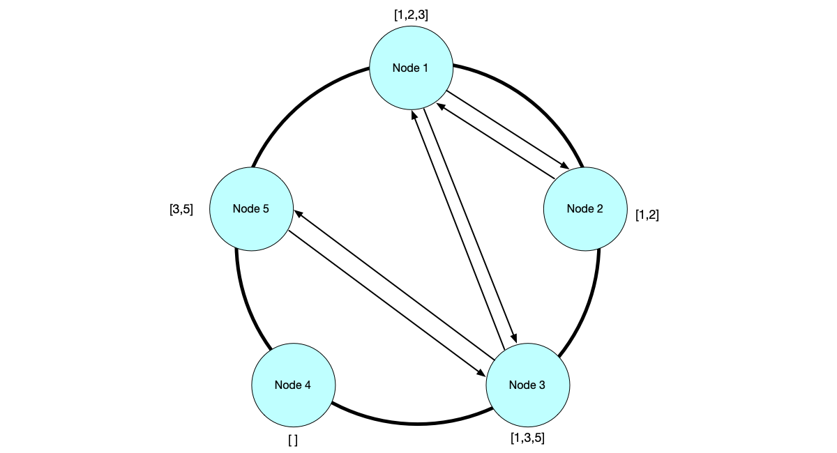
The gossip protocol brings significant advantages to Dynamo, while also having some limitations. For large-scale distributed systems like Dynamo, the decentralized nature of the gossip protocol makes it an ideal choice for managing cluster members.

Its main advantages are:

• High availability and fault tolerance: The decentralized architecture of the gossip protocol avoids single-point-of-failure problems. Even if some nodes fail, the cluster can still operate normally. Nodes randomly select communication partners, allowing information in the network to propagate through multiple paths, enhancing the system’s fault tolerance.
• Low communication overhead: Compared with traditional flooding mechanisms, the gossip protocol greatly reduces redundant messages in the network by randomly selecting communication partners. Dynamo’s gossip protocol only requires one random node communication per second, balancing real-time performance and network overhead, making it suitable for large-scale cluster environments.
• Elastic scalability: The propagation speed of the gossip protocol has a logarithmic relationship with network scale. It can remain efficient even in clusters with thousands of nodes. Dynamo achieves cluster expansion without central nodes through the gossip protocol. Nodes can join or leave the cluster at any time without affecting overall service.
• Fast convergence: The exponential propagation characteristic of the gossip protocol allows information to quickly diffuse throughout the entire cluster. In Dynamo, even if nodes change frequently, the cluster can reach a consistent view of membership status in a relatively short time, ensuring stable system operation.

However, the gossip protocol also has some limitations:

• Eventual consistency: The gossip protocol cannot guarantee strong consistency, only eventual consistency. In Dynamo, nodes may need some time to obtain the latest membership status, which may lead to brief inconsistency phenomena.
• Potential network storms: Although the gossip protocol reduces network overhead by randomly selecting communication partners, in large-scale clusters, frequent node changes may still trigger brief communication peaks. Dynamo effectively alleviates this problem by controlling gossip propagation frequency and adopting rumor propagation mode.
• Complexity of status synchronization: The gossip protocol needs to handle version conflicts and status inconsistency problems between nodes. Dynamo resolves version conflicts in membership status synchronization through vector clocks and “seen sets” mechanisms, but this also increases protocol complexity.

Since Dynamo’s release, the gossip protocol has been widely applied and improved in the distributed systems field. Modern distributed systems such as Cassandra, Riak, and Akka Cluster have all adopted gossip protocols similar to Dynamo for cluster membership management.

Data Repair #

Due to the leaderless architecture, write requests are not forced to be processed on all nodes before responding. Therefore, it may occur that the client is responded to before some nodes have successfully replicated. At this point, a data repair process is needed.

In the Dynamo architecture, nodes periodically and randomly select partners to “reconcile” with each other. If a node is found to have missing data, this portion of data needs to be synchronized to the failed node. This process of repairing data differences between nodes is called “anti-entropy.” A brute-force comparison of all key-value pairs between nodes is highly inefficient for large datasets. To quickly detect inconsistencies between replicas and minimize the amount of data recovered, Dynamo adopts the Merkle tree [26] [27] data structure. It is essentially a binary tree, where each node on the tree stores a hash value:

• If it is a leaf node: the hash value is the hash value of the value corresponding to the key.
• If it is a non-leaf node (i.e., internal node): the hash value is the value obtained by performing a hash calculation again on the hash values of its child nodes.

The figure below shows an example of a Merkle tree. In the figure, $h$ represents the hash function used, and $H$ represents the hash value calculated by the hash function. $H$ has two subscript representations depending on the node type:

• For leaf nodes, $H$ has only one subscript. For example, $H_1 = h(V_1)$ calculates the hash value of the value $V_1$ of leaf node 1.
• For non-leaf nodes, $H$ has two subscripts representing the data range of its child nodes. For example, $H_{12} = h(H_1 + H_2)$ represents the hash value of the sum of the hash values of child nodes $H_1$ and $H_2$.

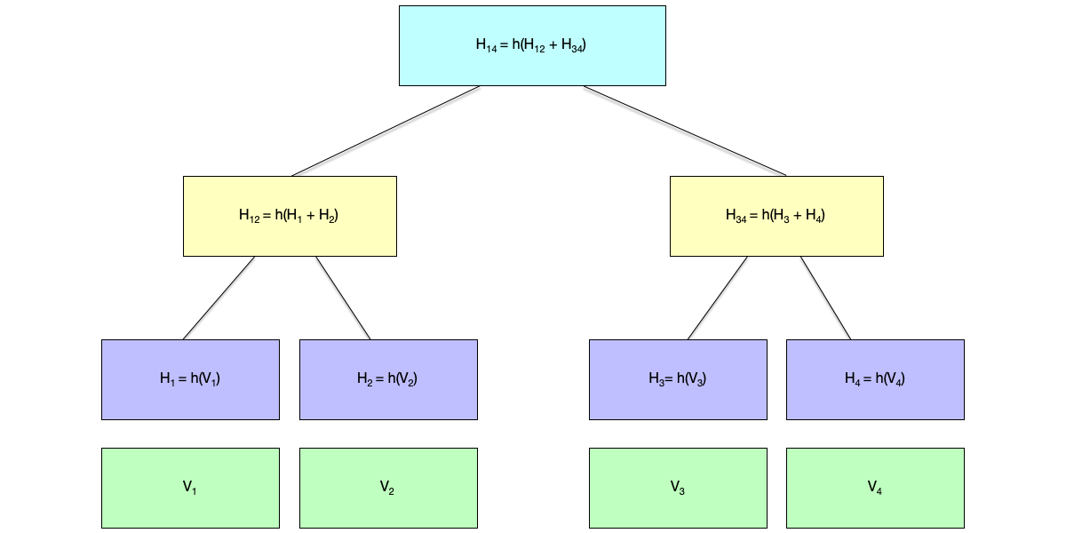
We can see that because the Merkle tree is a binary tree, the hash values of nodes are calculated from the bottom up. The following process can be used to compare whether the values of leaf nodes on two Merkle trees are the same:

• If the root node hash values of the two trees are the same, it means that the leaf nodes of the two trees must be the same.
• Otherwise, starting from the root node, traverse downward along nodes with different hash values to find all leaf nodes with different values. This process is the same as the binary tree search algorithm, with a time complexity of $O(\log_2(n))$. If a linear data structure (such as a linked list) is used to find data conflicts, a time complexity of $O(n)$ is required.

Each node in Dynamo maintains a separate Merkle tree for each virtual node covering the key range. When data needs to be recovered, the inconsistent leaf nodes can be immediately located for data synchronization according to the above process.

---

Amazon’s paper was published in 2007 and is a foundational work in the NoSQL and eventual consistency fields. Although there were already many NoSQL [28] databases before this, this paper, born from the production practice of the world’s largest e-commerce website, undoubtedly made the industry start thinking about two questions: whether SQL query functionality is needed, especially complex multi-table JOIN queries, which are not used in many scenarios. In addition, after the explosive growth of Internet users, system availability became a higher consideration. To guarantee system availability, strong consistency needs to be sacrificed. In this process, how should data conflicts be resolved?

Chapter Summary #

This chapter systematically explored one of the most core strategies in distributed systems—data replication. Starting from the basic goals of replication, we elaborated on its significant importance in high availability, fault tolerance, reduced latency, and improved read performance. However, the introduction of replication also brings the most thorny challenge in distributed systems: how to maintain consistency of multi-replica data in unreliable networks and node failures.

First, we detailed the primary-backup replication architecture, analyzing the trade-offs between synchronous, asynchronous, and semi-synchronous replication in terms of performance and data safety. For node failures and split-brain problems in primary-backup architecture, we discussed the key roles of heartbeat detection, lease mechanisms, and fencing tokens in guaranteeing system liveness and safety.

Subsequently, the focus of this chapter shifted to the theoretical system of consistency models. From the observer’s perspective, we defined linearizability, sequential consistency, causal consistency, and eventual consistency in order from strong to weak. By introducing the concepts of “safety” and “liveness,” we clarified that strong consistency belongs to strict constraints on system state, while eventual consistency is a promise of system convergence ability. At the same time, combined with the CAP theorem and its evolved version PACELC, from a theoretical height, we pointed out the irreconcilable contradiction between consistency and availability under network partitioning and latency constraints, providing a theoretical basis for system architecture selection.

For the user experience challenges that eventual consistency systems may bring, this chapter supplemented the introduction of client-centric consistency models (such as read your writes, monotonic reads, consistent prefix, etc.). Through the vivid case of a baseball game, we demonstrated how to use session-level consistency guarantees to satisfy the correctness of business logic without pursuing strong consistency, based on the needs of different business roles.

Finally, we turned to the decentralized leaderless replication architecture and analyzed the classic case of Amazon Dynamo. Through explanations of key technologies such as read-write quorum ($W+R>N$), vector clocks for handling concurrent conflicts, gossip protocol for cluster membership management, and Merkle tree for anti-entropy data repair, we demonstrated how to build an always-writable, highly available, and linearly scalable distributed storage system.

In summary, there is no absolute “silver bullet” for replication design in distributed systems. Whether choosing primary-backup architecture or leaderless architecture, or choosing strong consistency or eventual consistency, the essence is a game and trade-off between data consistency, system availability, and access latency. Understanding the principles and applicable scenarios behind these models is the cornerstone of building reliable distributed systems.

References #

1. Yoshinori Matsunobu: “Semi-Synchronous Replication at Facebook,” yoshinorimatsunobu.blogspot.com, 2014.

2. Michael Whittaker, Aleksey Charapko, Joseph M. Hellerstein, Heidi Howard, Ion Stoica: “Read-Write Quorum Systems Made Practical,” 2021.

3. etcd: “How To Watch Keys”

4. Jay Kreps: “I Heart Logs,” O’Reilly Media, 2014.

5. Redis: “Sentinel Documentation”

6. ACM Queue: “A Conversation with Bruce Lindsay,” ACM Queue, 2004.

7. Wikipedia: “Consistency Model”

8. Leslie Lamport: “How to Make a Multiprocessor Computer That Correctly Executes Multiprocess Programs,” IEEE Transactions on Computers, volume 28, number 9, pages 690–691, September 1979.

9. Maurice P. Herlihy and Jeannette M. Wing: “Linearizability: A Correctness Condition for Concurrent Objects,” ACM Transactions on Programming Languages and Systems (TOPLAS), volume 12, number 3, pages 463–492, July 1990.

10. Leslie Lamport: “On Interprocess Communication,” Distributed Computing, volume 1, numbers 2 and 3, 1986.

11. Douglas B. Terry, Alan J. Demers, Karin Petersen, Mike Spreitzer, Marvin Theimer, and Brent Welch: “Session Guarantees for Weakly Consistent Replicated Data,” at 3rd International Conference on Parallel and Distributed Information Systems (PDIS), September 1994.

12. Werner Vogels: “Eventually Consistent,” ACM Queue, 2007.

13. Werner Vogels: “Eventually Consistent — Revisited,” allthingsdistributed.com, 2008.

14. Wikipedia: “Safety and Liveness Properties”

15. Bowen Alpern and Fred B. Schneider: “Defining Liveness,” Information Processing Letters, volume 21, number 4, pages 181–185, October 1985.

16. Wikipedia: “CAP Theorem”

17. Eric A. Brewer: “Towards Robust Distributed Systems,” at ACM PODC Keynote, 2000.

18. Seth Gilbert and Nancy Lynch: “Brewer’s Conjecture and the Feasibility of Consistent, Available, Partition-Tolerant Web Services,” ACM SIGACT News, volume 33, number 2, pages 51–59, June 2002.

19. Eric A. Brewer: “CAP Twelve Years Later: How the Rules Have Changed,” infoq.com, 2012.

20. Daniel J. Abadi: “Problems with CAP, and Yahoo’s Little Known NoSQL System,” dbmsmusings.blogspot.com, 2010.

21. Martin Kleppmann: “A Critique of the CAP Theorem,” 2015.

22. Doug Terry: “Replicated Data Consistency Explained Through Baseball,” ACM Queue, volume 11, number 5, pages 28–37, May 2013.

23. David K. Gifford: “Weighted Voting for Replicated Data,” at 7th ACM Symposium on Operating Systems Principles (SOSP), 1979.

24. Giuseppe DeCandia, Deniz Hastorun, Madan Jampani, et al.: “Dynamo: Amazon’s Highly Available Key-value Store,” at 21st ACM Symposium on Operating Systems Principles (SOSP), October 2007.

25. Werner Vogels: “A Decade of Dynamo,” allthingsdistributed.com, 2017.

26. Ralph C. Merkle: “A Digital Signature Based on a Conventional Encryption Function,” in Advances in Cryptology — CRYPTO ‘87, LNCS 293, pages 369–378, 1987.

27. Wikipedia: “Merkle Tree”

28. Wikipedia: “NoSQL”