In distributed systems, multiple nodes work together. Client requests are sent to different nodes for processing, and these requests become events on individual nodes. As we will see, the system’s state is formed by executing these events one by one in a specific order. Therefore, the order of events is particularly important. Different nodes may see different sequences of events, which can lead to different states on these nodes.

From this, it is evident that when processing multiple events, the order in which they occur affects the state of nodes. Thus, how to measure the order of events becomes a core problem in distributed systems. A natural idea is to sort events according to their physical time. In the following sections, we will learn about the principles of physical clocks and, unfortunately, discover that in a distributed system, comparing physical time across multiple nodes to determine the order of events is not precise and can sometimes even lead to errors. Once the order of events is disrupted, the state of the entire distributed cluster becomes corrupted.

If physical time is not feasible, what other method can be used to determine the order of events in a distributed system? The answer is logical clocks.

Surprisingly, although we have repeatedly emphasized that the order of events is particularly important, in distributed systems there may still be cases where the order of occurrence of two events cannot be determined. Such events are called “concurrent events.” To explain event ordering, we also need to understand two mathematical definitions: partial order and total order. In fact, these two mathematical definitions should be deeply rooted in the mind of every distributed systems engineer, and we will encounter their applications in distributed systems again and again in later chapters.

---

In this chapter, we will discuss the following topics:

• How the order in which events occur affects the state of the system;
• Why physical time cannot be used to measure the order of events in distributed systems;
• The theoretical foundation and computation rules of logical clocks;
• Intuitive explanations and definitions of partial order and total order;
• Vector clocks, an extension based on logical clocks.

State, Events, and Snapshots #

In some crime dramas, we often see scenes like this: police are tracking a suspect who suddenly changes their behavior one day, so the police pull up records to review where the suspect went, who they met, and what they did over the past day, in order to understand what caused the suspect’s change.

Here, “places visited, people met, and things done” are individual events. If we view the suspect as a system, the suspect from yesterday and the suspect after these events represent the system’s states at different points in time. (From this, we might ponder a philosophical question, as shown below: the “me” of the past, after going through a series of events, becomes the “me” of the present—are these two “me’s” the same “me”?)

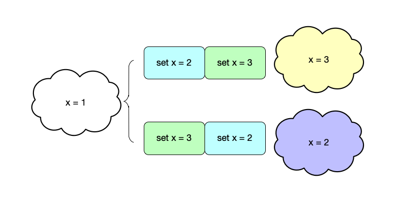
Let us continue explaining state and events with a simple storage service. As shown below, a storage service initially has state $\{x = 1\}$. After sequentially executing commands $set\ x = 2$ and $set\ x = 3$, the new state becomes $\{x = 3\}$. Here, the execution order of these two commands is particularly important; if the order of these two events is reversed, the resulting state becomes $\{x = 2\}$.

From the examples above, we can also see that we have not mentioned the physical time of event execution, but rather focus more on the order of event execution. The reason for focusing on the relative order between events rather than physical time is that there is no globally unified physical time in a distributed system. If we view the system as a large state machine, events are the operations that change the state of this state machine. In a state machine, as long as we can guarantee that events are executed in the same order every time, we can ensure that the system always reaches the same state.

Executing the same events in the same order produces the same result—this is the core idea of state machine replication [1]:

If two different processes start from the same initial state and process input data in the same order, they will produce the same output.

Note: After discussing logical clocks, we will see that the execution order of events is, in a sense, logical time.

On the other hand, the instantaneous state of this storage at different points in time is called a snapshot at that point in time. For example, taking a photograph on a busy street captures a snapshot of that street at that exact moment. In contrast, events are dynamic data used to change the system state, while snapshots are static data representing the system state.

At this point, we can give intuitive explanations of state, events, and snapshots:

• State: all data values in a system; state changes with events;
• Event: an operation that can change the system state. In a service, all write requests (writes, updates, deletions, etc.) can be called events;
• Snapshot: a snapshot is a special kind of state; it is a static state. Once the time of the snapshot is determined, its content is also determined.

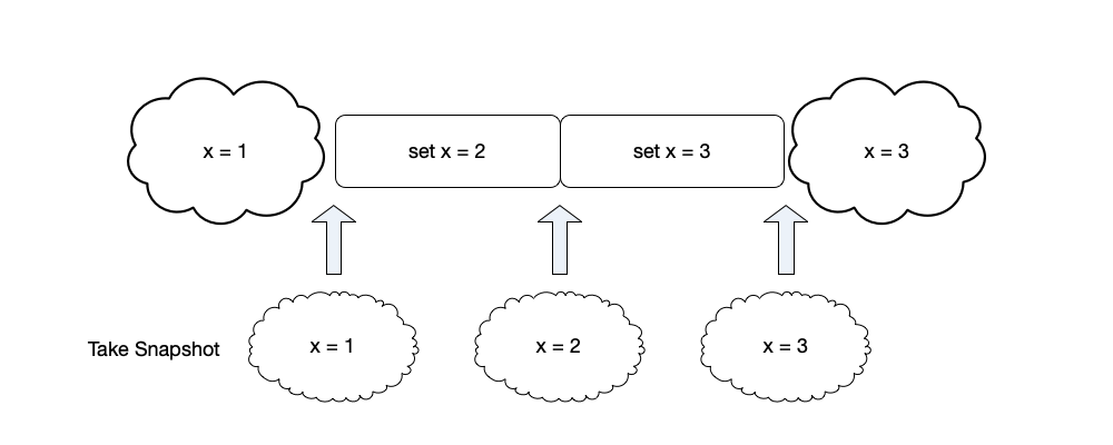
As shown in the figure below, if we obtain snapshots of the system at the initial time, after executing command $set\ x = 2$, and after executing command $set\ x = 3$, we will obtain $\{x = 1\}$, $\{x = 2\}$, and $\{x = 3\}$ respectively.

From the above explanations of state, events, and snapshots, we can see that these concepts are all strongly related to time, especially the relationship between events and temporal order. Next, we will look at how to measure the order of events on different nodes in a distributed system.

Note: Dividing the data related to a system into three categories—state, events, and snapshots—is also the approach used in data replication in distributed systems. Here we emphasize that in distributed systems, maintaining the same order of events across multiple replicas is required; a stronger requirement than this is determinism. We will also see in the consensus algorithms chapter that consensus algorithms are essentially log systems maintaining the same order across multiple replicas.

Physical Clocks #

Physical Time Sources and Representation #

Most computer clocks today use quartz clocks. Quartz clocks are usually powered by batteries, with a quartz crystal (typically in a tuning-fork shape) at their core. When voltage is applied to the quartz crystal, it generates mechanical vibrations due to the piezoelectric effect, with a very stable frequency (usually 32,768 Hz). This high-precision oscillation is the foundation of quartz clock timing. After a predefined number of oscillations, the timer chip inside the computer interrupts once (called a clock tick). The interrupt handler increments a counter that records the number of ticks since some past epoch. Knowing the number of ticks per second, we can calculate the year, month, day, and time.

Quartz clocks are inexpensive but not accurate enough. Due to manufacturing differences, each quartz crystal has a slightly different oscillation frequency. Additionally, quartz crystals operate at room temperature, and temperature increases or decreases change their vibration frequency. Since every computer has a quartz clock, these differences in oscillation mean that clocks in different computer hosts may drift—one node may run slow while another runs fast.

Quartz clocks may have their vibration frequency altered by environmental factors, causing the clock’s running speed to change. So, is it possible to find a substance that can vibrate at a constant frequency? If so, time could be represented as the number of vibrations of this substance. In the 1930s, Isidor Isaac Rabi [2] and his students at Columbia University’s laboratory studied the fundamental properties of atoms and atomic nuclei. They eventually discovered that the resonance frequency of certain atoms is extremely accurate and could be used to build highly precise clocks. Atomic clocks [3] are timing devices based on atomic resonance: they are built on the principles of quantum mechanics and represent the most precise timing technology humans have mastered, with an error of only one second over millions of years. This extreme precision stems from the electromagnetic wave frequency radiated when electrons inside atoms transition between specific energy levels. This frequency has extremely high stability and is almost completely immune to external environmental disturbances such as temperature and pressure.

In fact, International Atomic Time (TAI) [4] is based on this principle to define the standard unit of time: 1 second is defined as the duration of 9,192,631,770 periods of the radiation corresponding to the transition between two hyperfine levels of the ground state of the cesium-133 atom. Although atomic clocks are expensive, their unparalleled accuracy has made them indispensable infrastructure for scientific research, modern communications, and global positioning systems (GPS).

Atomic clocks seem to work very well, but they ignore the astronomical concept of time. People’s perception of a day is based on sunrise and sunset. In astronomical terms, a “day” refers to the time it takes for the Earth to rotate once. Due to factors such as tides, earthquakes, and glacier changes, the Earth’s rotation speed is not constant. For example, on August 5, 2025, the Earth’s rotation speed increased, making it the shortest day on record [5]. This day was 1.25 milliseconds shorter than 86,400 seconds.

From this perspective, on the question of “how long is a day,” we encounter two different definitions: one based on the quantum mechanics mechanism of atomic clocks, and the other based on astronomy. These two definitions do not always match precisely.

To solve this problem, Coordinated Universal Time (UTC) [6] was introduced in 1972. It is based on atomic clocks and defines the world time standard, consisting of two parts:

• Atomic time TAI, which is the weighted average of hundreds of atomic clocks worldwide.
• It is based on atomic time and uses micro-adjustments to stay roughly synchronized with Universal Time (UT).

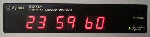
To keep UTC within 0.9 seconds of mean solar time, the International Earth Rotation and Reference Systems Service (IERS) inserts or deletes leap seconds [7] as needed. Leap seconds are usually implemented on the last second of June 30 or December 31, adjusting UTC time to 23:59:60. This adjustment allows UTC to maintain the precision of atomic time while roughly synchronizing with the “solar time” of Earth’s rotation. If a leap second adjustment is needed, the relevant institutions announce the adjustment time for the following year one year in advance. For example, in December 2016, the National Time Service Center of China issued the “Leap Second Announcement”, stating:

On July 6, 2016, the Paris-based International Earth Rotation Service (IERS) issued a leap second announcement in its Bulletin C 52 to global institutions responsible for standard time measurement and dissemination: the international standard time UTC (Coordinated Universal Time) will implement a positive leap second on January 1, 2017, adding 1 second. On July 11, the Time Department of the International Bureau of Weights and Measures (BIPM) issued a leap second adjustment forecast to global timekeeping laboratories participating in the International Atomic Time (TAI) calculation. Due to time zone differences, China will synchronize the leap second adjustment with the world at 07:59:59 Beijing time on January 1, 2017, resulting in the special phenomenon of 07:59:60.

Note: The abbreviation for Coordinated Universal Time is UTC, which is clearly not an acronym for “Coordinated Universal Time.” Behind this is a story of compromise: the International Telecommunication Union wanted Coordinated Universal Time to have a single abbreviation in all languages. People in English and French-speaking regions both wanted their respective abbreviations—CUT and TUC—to become the international standard, and the final compromise was to use UTC.

In the military, the Coordinated Universal Time zone is represented by “Z.” In aviation, all times used are uniformly specified as Coordinated Universal Time. Moreover, Z should be read as “Zulu” in the NATO phonetic alphabet over radio, so Coordinated Universal Time is also called “Zulu time.” For example, if a plane takes off at 18:00 Beijing time (UTC+8), it would be written as 1000z, or read as “1000 Zulu.”

UTC unified the world time standard, and time zones in different countries and regions are also defined in terms of UTC. If the local time is ahead of UTC, for example, China’s time is 8 hours ahead of UTC, it is written as UTC+8, commonly known as the East Eighth Zone. Conversely, if the local time is behind UTC, for example, Hawaii’s time is 10 hours behind UTC, it is written as UTC-10, commonly known as the West Tenth Zone.

The appearance of leap seconds introduces complexity and potential problems for some computer programs. According to the concept of leap seconds, a day does not always have exactly 86,400 seconds; it may have 86,399 seconds (deleting a leap second) or 86,401 seconds (adding a leap second). Leap seconds bring new problems to time measurement in computer systems. To understand this, we first need to understand the clock system in computer systems.

Wall Clocks and Monotonic Clocks #

Modern computer systems have two clock systems: the wall clock and the monotonic clock. These two clock systems answer different questions. Understanding the difference between these two clock systems helps deepen the understanding of time issues in distributed systems.

---

Wall Clock

As the name suggests, the “wall clock” can be understood as a clock hanging on the wall; it answers the question “what time is it now?” The most commonly used Unix time [8] in the computer field represents the number of seconds elapsed since January 1, 1970. Under Linux, you can use clock_gettime(CLOCK_REALTIME) to obtain the system’s Unix time; similarly, Java provides System.currentTimeMillis() for the same purpose.

Unix time does not account for leap seconds, so any code using Unix time to measure time differences must additionally consider whether leap seconds need to be taken into account. Historically, leap seconds have caused many major failures in the Internet domain. For example, on June 30, 2012 [9], an extra second in global time caused chaos on the Internet. Mainstream platforms such as LinkedIn, Reddit, and Mozilla experienced partial outages, and countless Linux servers (including many servers from Red Hat, Debian, and Ubuntu vendors) saw CPU utilization spike to 100%, causing crashes. For more leap-second-related issues and failures, please refer to [10].

Note: From the definition of Unix time, we know that the unit of this time representation is seconds, but some APIs provide Unix time in other units. For example, Java’s System.currentTimeMillis() function provides the number of milliseconds elapsed since January 1, 1970.

In addition to the leap second problem, we will also see later that when using the NTP protocol for time synchronization, the wall clock can also jump backward.

---

Monotonic Clock

Unlike the wall clock, the monotonic clock answers the question of time difference, i.e., “how much time has passed.” It is like a stopwatch in a computer system, telling developers how long the system has been running. It represents the time elapsed since “some arbitrary point in time” (usually the moment the operating system boots). The absolute value itself (e.g., 43,567,890 nanoseconds) has no meaning; only the difference between two monotonic clock readings is meaningful.

Because the monotonic clock satisfies the property of monotonic increase, no matter how the NTP protocol adjusts the system time, the monotonic clock only moves forward and will not go backward. Even if the NTP protocol discovers that the local clock is running too fast, it will not simply roll the monotonic clock back; instead, it will subtly adjust the clock frequency (slewing) to make it run slightly slower until it catches up with the standard time, but the monotonic clock value will still increase.

It is important to emphasize that since the starting time of the monotonic clock is usually the operating system boot time, monotonic clocks on two different machines cannot be compared. That is, the monotonic clock cannot be compared across nodes.

With this understanding of the two clock systems, we can next look at how systems synchronize physical time.

Physical Time Synchronization #

Atomic clocks built on quantum physics are more accurate but expensive. To solve the problem of low time precision on computers, computers periodically synchronize time with high-precision time systems through clock synchronization protocols. NTP (Network Time Protocol) [11] is currently the most mainstream clock synchronization protocol; almost all personal computers, smart devices, and mobile devices use NTP for clock synchronization.

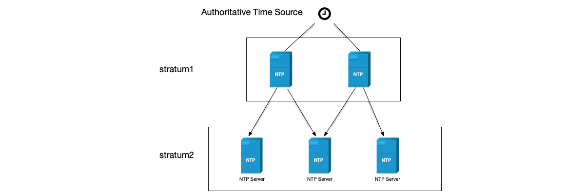
The NTP protocol organizes its structure in multiple layers, where each layer is called a stratum. The stratum number of an NTP server that obtains clock synchronization from the most authoritative clock is usually set to stratum 1, serving as the primary time server to provide clock synchronization for other devices on the network. Stratum 2 obtains time from stratum 1; similarly, stratum 3 obtains time from stratum 2, and so on. The clock stratum value ranges from 1 to 16; the smaller the value, the higher the time precision.

The NTP protocol is a typical client/server architecture protocol. After receiving a request from an NTP client, the NTP server responds with the current NTP server time to correct the NTP client time. Due to network delays, differences in CPU processing speed, and other reasons, to precisely synchronize the clock, the response sent to the NTP client needs to include the times when the server received and sent the response, so that the client can estimate the delay.

The following shows a complete NTP request process:

1. The client sends an NTP request packet to the server at time $t_1$, which includes the departure time $t_1$ of this packet from the client.
2. The NTP request packet arrives at the server at time $t_2$. After receiving and processing the packet, the server sends a response packet at time $t_3$. The response packet carries the departure time $t_1$ of the packet from the client, the time $t_2$ when the server received the request packet, and the departure time $t_3$ of the response packet from the server.
3. The client receives the response packet from the server at time $t_4$.

As can be seen, if we can calculate the delay time difference between the client and the server, then based on the server response time $t_3$, we can infer the current time at the client.

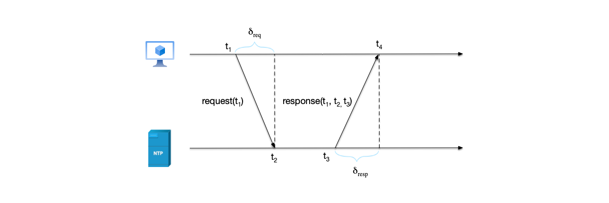
In the process above, there are two time differences related to network delay:

$$\delta_{req} = t_2 - t_1 \text{, request delay}$$$$\delta_{resp} = t_4 - t_3 \text{, response delay}$$

The total round-trip delay is the sum of the two:

$$\delta = \delta_{req} + \delta_{resp}$$

The NTP protocol assumes that the round-trip time difference divided by 2 is the delay time of one NTP message. Adding this time to the server response time $t_3$ gives the time at the NTP client. That is, the time $\theta$ that the NTP client should set after receiving the response is:

$$\theta = t_3 + \frac{\delta}{2} = t_3 + \frac{\delta_{req} + \delta_{resp}}{2}$$

Looking closely at the NTP time offset formula $\theta = t_3 + \frac{\delta}{2}$, we will find that this formula hides a huge assumption: the delay of the request and the delay of the response are equal, i.e., $\delta_{req} = \delta_{resp}$. The NTP protocol assumes that the network is symmetric: the outbound and return paths are the same and take the same amount of time.

However, in actual wide area network (public Internet) environments, this assumption is often not valid. This is network asymmetry:

• Different routing paths: The Internet’s complex routing strategies mean that the path of a data packet from A to B is often different from the path from B back to A. The outbound path may go over fiber optics, while the return path may take a detour or even go through congested links.
• Different bandwidth and queuing: Even if the paths are the same, the inconsistency between upstream and downstream bandwidth (such as common residential broadband ADSL or cloud server bandwidth limits) can cause the request and response to wait in router queues for vastly different amounts of time.

This asymmetry introduces an irremovable systematic error into NTP. If the request takes 100ms and the response only takes 10ms, NTP crudely assumes that each one-way trip is 55ms, which directly causes the calculated time $\theta$ to deviate by 45ms.

In addition, NTP’s stratum hierarchy further amplifies this uncertainty. A server at stratum 3 needs to synchronize from stratum 2, which in turn synchronizes from stratum 1. Synchronization at each level carries the risk of network asymmetry, and this error accumulates level by level. It is like a game of telephone: the more people the message passes through, the more distorted the “time” heard at the end.

It is precisely because of these unavoidable physical characteristics in physical networks that we can never obtain a truly accurate global physical clock in a distributed system.

In addition to errors, we must also see that as NTP clients, computers have their time adjusted by the NTP protocol. For example, at one point in time, the system clock is synchronized with NTP time, but at another point, due to network delays and other reasons, the estimated network delay differs from before, causing the system to suddenly jump forward or backward in time. This phenomenon of sudden forward or backward time adjustments in NTP clients can also cause problems in production. Cloudflare reported an incident in January 2017 [12]. The core cause of the failure was that some key logic relied on the result of time difference calculations without considering that time could be adjusted backward (i.e., without guaranteeing monotonicity).

From the above analysis, we can see that if we are only interested in measuring time differences (e.g., measuring request-response time differences), we can consider using a monotonic clock. The monotonic clock does not require global synchronization, always moves forward, and represents the duration since the host booted, so there will be no time rollback. In contrast, the wall clock synchronizes time with the NTP server and may jump backward after time calibration.

Deficiencies of Physical Clocks #

So far, we have learned about the several different sources of physical time in computer systems, two different physical clock systems, and the physical time synchronization mechanism. Physical time has two deficiencies: clock skew and clock drift, which make it impossible to use physical time to determine the order of distributed events in a distributed system.

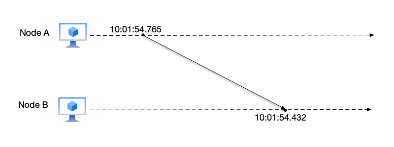
Clock skew refers to the time difference between the clocks of multiple devices. For example, in a distributed system, node A’s clock shows 12:00:00 while node B shows 12:00:01—this is the clock skew between these two nodes.

Due to clock skew, on different physical devices, we cannot determine the order of events by comparing their respective wall clock times. As shown below, a message sent by user A at local time 10:01:54.765 is received by user B at local time 10:01:54.432. To user B, it seems as if a message from the “future” has been received.

Clock drift refers to the difference in speed between a device’s local clock and standard time. Over time, the local clock’s timing speed may be slightly faster or slower, causing the gap with standard time to grow larger and larger. For example, a device’s clock may gain or lose a few milliseconds per day; after long-term accumulation, this may lead to minute-level deviations. To correct the device’s local clock, it needs to synchronize time with an NTP server. However, during time correction, the time may drift forward or backward.

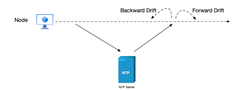
Since wall clock time may drift backward at random moments, wall clocks cannot be used to measure the time difference between two events in a system; monotonic clocks should be used instead.

At the same time, because different nodes synchronize and correct time with the NTP server, they may have inconsistent wall clock times due to various reasons (network, delay, the node’s own clock frequency, etc.). Therefore, in a distributed system composed of multiple nodes, there is no globally unique clock, and we cannot use physical time to measure the order of events as we would in a single-node system.

So, how do we solve the problem of event ordering in distributed systems? We need to re-examine the relationships between events in distributed systems.

Note: It is worth noting that although NTP and ordinary quartz clocks cannot meet the requirements of strongly consistent systems, hardware-assisted clock synchronization technology has made breakthrough progress in recent years. The most famous example is the TrueTime API used by Google Spanner. It uses GPS receivers and atomic clocks in data centers to compress clock errors into an extremely small millisecond-level range, and most critically—it can explicitly tell the caller the upper and lower bounds of this error.

This design of “incorporating the error of physical time into causal inference” allows Spanner to achieve external consistency without completely relying on logical clocks. TrueTime represents another philosophy of distributed system design: hardware and software co-design. We will explore this technology in depth when we discuss distributed transactions later. But before that, we need to first master the more universally applicable foundational tool: the logical clock.

Causality and Event Ordering #

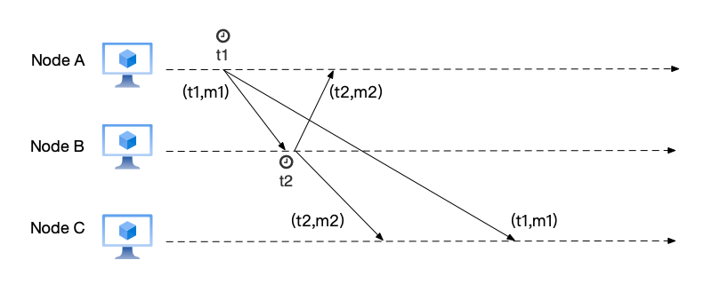
Having understood physical clocks, we now return to distributed systems and look at a typical problem. Here, message m1 is sent by user A and broadcast to users B and C, with the content “Where shall we go today?”; message m2 is a reply from user B after receiving message m1, broadcast to users A and C, with the content “Let’s go to the movies.”

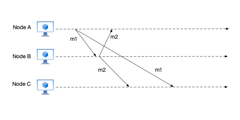
From the relationship between m1 and m2, the two are causally related: that is, user A’s question (message m1) comes first, and then user B’s response (message m2). However, user C first sees message m2 and then message m1. This order violates causality: because the response is seen before the question.

Let us change this to a more technical example. Suppose message m1 is an instruction to create a new object, and message m2 is an instruction to update this object’s value. Clearly, message m1 should occur before message m2, because the object must be created before its value can be modified. If the order of these two messages is reversed on some node, the update operation will fail because the message to create the object has not yet arrived, so the object does not yet exist on that node; and when the message to create the object is received and executed, the object’s value will never be updated because the instruction to update the object was already processed earlier.

Returning to the problem, we consider adding a timestamp to each message: the original protocol format was “(message body)”, and now it is changed to “(timestamp, message body)”. We attempt to solve the causal ordering problem here by adding timestamps to the protocol. So, how should this timestamp be chosen?

First, we rule out the monotonic clock option, because monotonic clock values cannot be compared across different nodes.

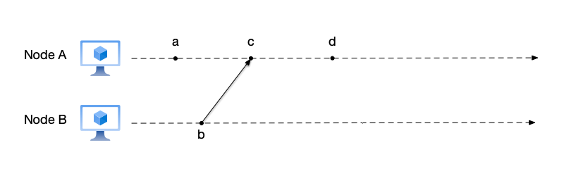
Using the wall clock also won’t work. Even if a protocol like NTP is used to synchronize time across different nodes, especially when network delays between different nodes and the NTP server are asymmetric, there is no guarantee that the wall clocks of multiple nodes will be consistent. As shown in the figure below, the time when user A sends message m1 is t1, and the time when user B sends message m2 is t2. Here, we cannot guarantee that time t1 on A must be less than time t2 on user B. Therefore, if the wall clock is used to order events, errors may still occur.

In 1975, Paul Johnson and Bob Thomas published a paper [13], also attempting to solve the above problem with timestamps. Leslie Lamport [14] quickly discovered the problem in the paper. In Lamport’s own words:

I realized that the essence of Johnson and Thomas’s algorithm was the use of timestamps to provide a total ordering of events that was consistent with the causal order.

Lamport wrote these insights into the paper “Time, Clocks, and the Ordering of Events in a Distributed System” [15]. Let us see how this paper solves the problem of event ordering.

In the paper, Lamport introduced the Happened-before relation [16], used to express the ordering of multi-node events in distributed systems. Event A happening before event B is denoted as $A \to B$. Its core idea is to divide events in a distributed system into the following three categories: local events, message send events, and message receive events, and to define precedence among these three categories of events.

The following are the three conditions that define the Happened-before relation:

1. Local events: if events A and B occur sequentially on the same node, then $A \to B$.
2. Send message event: if event A is a message send event on one node, and event B is the corresponding message receive event on the receiving node, then $A \to B$. This is because causally related events must have an order: the cause (message send event) comes before the effect (message receive event).
3. Satisfies transitivity: for three events A, B, and C, if both $A \to B$ and $B \to C$ hold, then $A \to C$ also holds.

If for two events A and B, neither $A \to B$ nor $B \to A$ holds, then these two events are called concurrent events, denoted as $A \| B$. In mathematical language, concurrent events are expressed as:

$$a \| b \iff \neg (a \to b) \land \neg (b \to a)$$

From the three conditions of Happened-before above, it can be seen that two concurrent events must be located on different nodes, and there is no message passing between them. Because there is no message passing, their order relationship cannot be confirmed.

Taking the figure above as an example to explain event ordering, the line and arrow between events b and c in the figure indicate that they are the send and receive events of the same message:

• According to rule 1, events a, c, and d occur sequentially on node A, so $a \to c$, $c \to d$;
• According to rule 2, event b is the message send event on node B sending a message to node A, and event c is the corresponding message receive event on node A, so $b \to c$;
• According to rule 3, $a \to d$, $b \to d$;
• For events a and b, neither $a \to b$ nor $b \to a$ holds, so they are concurrent events.

Let us expand the figure above by introducing several nodes called “observers.” These observer nodes can see events on nodes A and B, and sort these events on the same observer node’s timeline, which is equivalent to “merging” the event timelines of multiple nodes onto the observer node’s timeline.

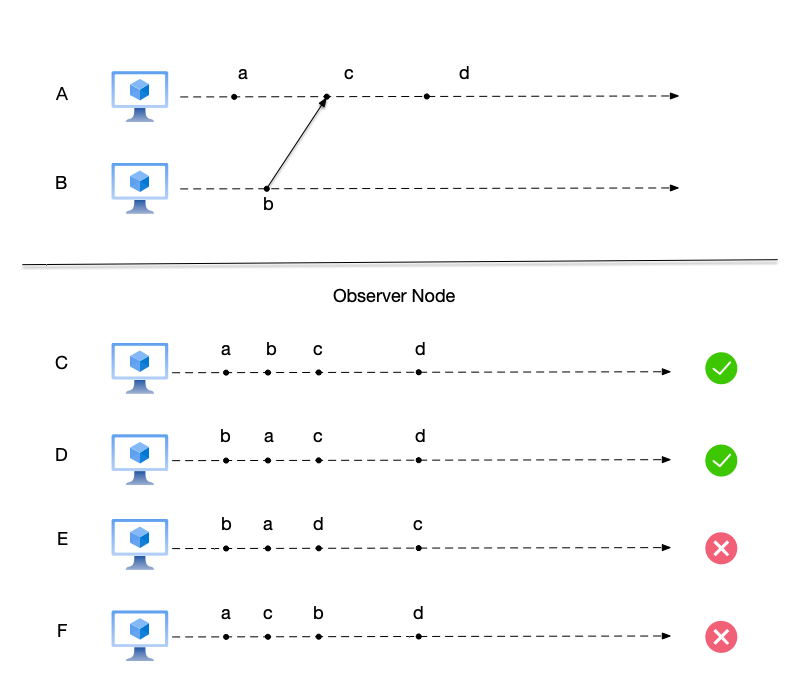
In the figure above:

• Node C observes the event sequence (a,b,c,d); this ordering does not violate the Happened-before relation.
• Node D observes the event sequence (b,a,c,d); this ordering does not violate the Happened-before relation.
• Node E observes the event sequence (b,a,d,c); here event d is placed before event c. We have already mentioned earlier that these two events satisfy $c \to d$, so this ordering is incorrect.
• Node F observes the event sequence (a,c,b,d); here event c is placed before event b. We have already mentioned earlier that these two events satisfy $b \to c$, so this ordering is incorrect.

It is worth explaining here: the difference between node C and node D is how events a and b are ordered. As mentioned earlier, these two events are concurrent events. In some consistency models, different nodes may arrange concurrent events in any order without causing data corruption; we will return to this discussion when we talk about consistency models later.

Note: Social media products can be used to understand the “merging” operation above. Observer nodes and nodes that produce events are equivalent to accounts on social media. Each observer account follows multiple accounts (nodes A and B in the above example). These accounts post different messages on their own timelines, but from the perspective of their followers, these messages ultimately need to be aggregated and have a reasonable ordering on the follower’s own timeline.

For concurrent events, the order seen on the same account can be arranged arbitrarily, but for events satisfying the Happened-before relation, their order must be guaranteed.

Total Order and Partial Order #

In the previous section, we introduced the Happened-before relation for events. There also exist concurrent events that do not satisfy this relation. To understand these relationships more deeply, we need to understand two mathematical concepts: partial order [17] and total order [18].

Many engineers feel intimidated when they see mathematical definitions, but in fact, these two concepts are everywhere in our daily lives. Before entering strict mathematical descriptions, let us first use two life scenarios to build intuitive understanding.

---

Total Order: The Line at a Bank Counter

Imagine you are standing in line at a bank counter to conduct business. People stand in a sequence. For any two people in the line (say, Alice and Bob), we can definitely determine their order:

• Either Alice is in front of Bob;
• Or Bob is in front of Alice.

This property, where any two elements can be compared, defines a total order. In a single-node system, because there is only one CPU clock, all events are like people in a line: their absolute order can always be determined. Therefore, single-node events usually satisfy a total order relationship.

---

Partial Order: The Reporting Structure of a Company

Now, let us switch the scenario to the organizational chart of a large company. We define a relationship called “reports to” (i.e., a subordinate reports to a superior).

• Vertical comparison (comparable): Programmer Tim reports to the tech manager, and the tech manager reports to the CTO. In this chain, we can clearly say: “Tim is ‘below’ the CTO in the hierarchy.” This relationship is clear.
• Horizontal comparison (incomparable): Now let us use this “reports to” relationship to compare the tech manager and the finance manager. You will find that they cannot be compared—the tech manager does not report to the finance manager, and the finance manager does not report to the tech manager. They work in parallel in their respective departments, with no subordination between them.

In this system, only “some” members have a clear hierarchical relationship, while other members (such as managers of the same level in different departments) cannot be compared through this relationship. This relationship of “order exists only among some members, and members that cannot be compared concurrently are allowed” is the partial order.

Mapping to distributed systems:

• Reporting relationship $\Longleftrightarrow$ Happened-before.
• Cross-department managers with no subordination $\Longleftrightarrow$ concurrent events.

Understanding this, let us now see how mathematicians describe these two types of relationships in rigorous language.

---

Partial Order

A partial order represents a binary relation R in which only some members of the set can be compared using this binary relation. The binary relation R used to compare set members must satisfy the following three rules in mathematics:

1. Reflexivity: for any member $x$ in the set, $xRx$ holds;
2. Antisymmetry: for any members $x$ and $y$ in the set, if $xRy$ and $yRx$ hold, then $x = y$;
3. Transitivity: for any members $x$, $y$, and $z$ in the set, if $xRy$ and $yRz$ hold, then $xRz$ holds.

Let us give an example to understand partial order. For the set $\{a, b, c\}$, the set of all its subsets is $\{\{\},\{a\}, \{b\}, \{c\}, \{a, b\}, \{a, c\}, \{b, c\}, \{a, b, c\}\}$. All these members are subsets of the original set and can be related through the $\subseteq$ relation:

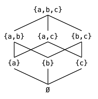
We note that the $\subseteq$ relation here satisfies the three rules above. However, not all members here satisfy the $\subseteq$ relation with each other; for example, $\{a, b\} \nsubseteq \{b,c\}$ and $\{b,c\} \nsubseteq \{a,b\}$.

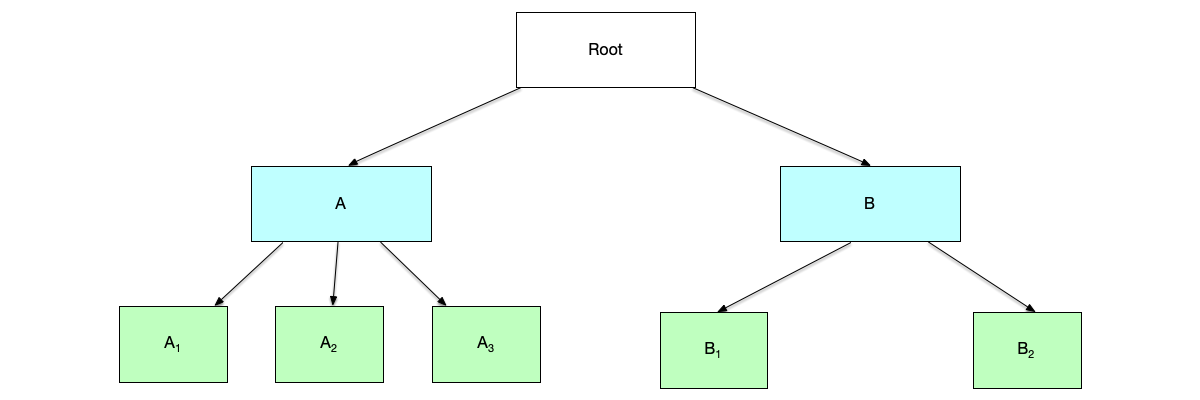
Tree relationships are also a common form of partial order. In the tree shown below, nodes at the same level cannot be compared in size, because in terms of the “level” relationship, nodes at the same level are the same; for example, node A and node B have the same level.

---

Total Order

On the other hand, if all members of a set can be compared using a binary relation, this binary relation is called a total order relation. Formally, a total order relation adds a totality constraint on top of a partial order relation. That is, a total order relation $R$ requires satisfying the following four rules:

1. Reflexivity: for any member $x$ in the set, $xRx$ holds;
2. Antisymmetry: for any members $x$ and $y$ in the set, if $xRy$ and $yRx$ hold, then $x = y$;
3. Transitivity: for any members $x$, $y$, and $z$ in the set, if $xRy$ and $yRz$ hold, then $xRz$ holds.
4. Totality: for any members $x$ and $y$ in the set, either $x \leq y$ or $y \leq x$ holds.

For example, any two elements in the set of integers can be compared using the binary relation $\leq$, and this relation is a total order relation for this set.

We can see that the difference between partial order and total order is: partial order requires elements in the set to be partially ordered, while total order requires elements in the set to be totally ordered.

From the above explanations of total order and partial order, we can see that the Happened-before relation is a partial order relation. Those concurrent events are events whose order cannot be compared.

Note: However, the Happened-before relation does not satisfy reflexivity, because for an event A, one cannot say “A happened before A.” So in the strict sense, the Happened-before relation is called an irreflexive partial order. For simplicity, we will still consider the Happened-before relation as a partial order relation later and will no longer specifically emphasize the violation of reflexivity.

On a single-node system, because there is a unique global clock, events on the system occur sequentially in time order; one event ends before the next event occurs. Therefore, it is easy to perform a total ordering of events on a single-node system. However, on a distributed system, performing a total ordering of events is very difficult. There are two reasons:

1. Events on multiple nodes occur concurrently;
2. There is no global clock in a distributed system; instead, each node has its own clock.

Taking the figure below as an example, we represent events using start and end times as “[start time, end time].” We can see that in a single-node system, events execute sequentially and satisfy a total order relationship; in a distributed system, events on multiple nodes execute concurrently. For example, event [1,3] on node A and event [2,4] on node B do not satisfy a total order relationship.

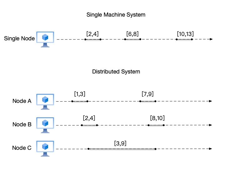
The figure above also implies an assumption: there exists a global clock for the distributed system, and all nodes in the system can record the start and end times of events based on this global clock. In reality, maintaining this global physical clock for each node is generally handled by services like NTP. However, considering the network delay between each node and the NTP service, as well as the operating conditions of the nodes, the time synchronization between this global clock and each node has different errors. Therefore, on a distributed system, there is no global clock; instead, each node has its own clock. This is the second reason why global ordering is difficult on a distributed system.

In daily life, we are already accustomed to the events around us being totally ordered. For example,

• Waiting in line to buy movie tickets, or waiting to pass through a traffic light;
• When shopping, first putting items into the shopping cart, then checking out.

However, when it comes to multi-person interactions, there are many scenarios where it is difficult to totally order events, such as:

• In a group chat, multiple users are speaking. The order of these messages may be different in different accounts;
• Multiple comments on the same post on social media may also not have a single ordering.

The reason people are accustomed to the events around them being ordered is mainly due to the single perspective of an individual. But from a distributed perspective, not all events occurring on different nodes are ordered.

We will see later in the consistency model chapter that in many scenarios there is no need to implement a total order relationship. Maintaining a total order relationship among events comes at a great cost: more resource consumption, less event concurrency, and so on. On the contrary, in many cases, implementing causal consistency is sufficient—that is, only maintaining the order for causally related events, while concurrent events among multiple nodes can be ordered arbitrarily.

Causality and the Happened-before Relation #

Causality in real life is determined based on loosely synchronized clocks (watches, wall clocks) under the illusion that a global clock exists. For example,

• Making time plans: plan to arrive at the station at 6:10 to catch the 6:30 bus;
• Alibi [19]: if a suspect appears in a video at some location at 6:00, then they cannot have committed a crime ten kilometers away at 6:10.

In these life scenarios, the requirements for time precision are relatively coarse, tolerating errors of several seconds or even tens of seconds. This is because in real life, information flows slowly, so small clock errors do not cause serious problems. But in a distributed system, events occur at higher frequencies and speeds, and the duration of events is many orders of magnitude shorter than events in real life. If the physical clocks in a distributed system are not precisely synchronized, it is difficult to determine the causal relationships between events.

Let us review the three situations that satisfy the Happened-before relation. The second situation implicitly contains causality: the message send event is the cause, and the message receive event is the effect. Happened-before is a way to reason about causality in distributed systems. In the second situation of Happened-before, it considers whether information flows from one event to another, which indicates whether one event may affect another. Therefore, the Happened-before relation can conveniently express causality between events: if event A causes event B, then event A must have happened before event B.

But the other two situations of Happened-before do not necessarily imply causality. Situation one says that events occurring sequentially within the same node have a Happened-before relationship; situation three says that the Happened-before relation is transitive. In these two situations, events satisfying the Happened-before relationship do not necessarily have a causal relationship. Therefore, we say that if event A happened before event B, then event A might have caused event B.

Finally, for concurrent events, there must be no causal relationship. For example, events a and b in the earlier figure.

To summarize, causality and the Happened-before relation have the following three relationships:

• If event A causes event B, then event A must have happened before event B (if event A causes event B, then $A \to B$);
• If event A happened before event B, then event A might have caused event B (if $A \to B$, then A might cause B);
• For two concurrent events, there is definitively no causal relationship (if $A \| B$, then event A MUST NOT cause event B, and event B MUST NOT cause event A).

Note: Please note in the above statements which ones use might and which ones use must.

Logical Clocks #

Since physical time cannot be used as a basis for measuring the order of events in distributed systems, Lamport then introduced the concept of “logical clocks” in his paper to solve this problem.

A logical clock can be understood as a counter, with each event corresponding to a separate count. There are many ways to implement this count, but no matter which one, it must satisfy the following clock condition (let the logical clock function for events be C(e), where parameter e is the event):

If event a happens before event b, then $C(a) < C(b)$.

When explaining Happened-before earlier, we used the symbol $a \to b$ to denote that event a happens before event b. Therefore, the clock condition can be expressed in mathematical language as follows:

$$a \to b \Rightarrow C(a) < C(b)$$

Note that in logical clocks, the converse of the clock condition does not hold, i.e.:

If $C(a) < C(b)$, it is not certain that event a happens before event b.

In mathematical language:

$$C(a) < C(b) \nRightarrow a \to b$$

Note that “it is not guaranteed that event a happened before event b” means: it is possible that event a happens before event b, or the two events may be concurrent events. That is: $C(a) < C(b) \Rightarrow (a \to b) \lor (a\ \| b)$.

If both conditions above can be satisfied simultaneously, i.e., $a \to b \iff C(a) < C(b)$, this is called the “strong consistency condition”.

Note: The “consistency” in the strong consistency condition is different from the “consistency” in the “consistency models” we will mention later. The strong consistency condition means that there is a consistent relationship between logical time and event order: by comparing logical times, the order relationship between events can be derived; conversely, if the order relationship between events is known, the magnitude relationship of their logical times can also be determined.

Although there are many different logical clock implementations, in general, the implementation of logical clocks has two main parts [20]:

• The data structure used to represent the logical clock;
• The protocol used to update the logical clock representation when there is message passing between nodes.

Each node maintains the following data:

• The logical clock within the node, used to measure the order of events within this node;
• The global logical clock from the node’s perspective.

The protocol includes the following two rules:

• Rule 1: describes how to update the local logical clock when a node executes an event;
• Rule 2: describes how to update the global logical clock from this node’s perspective.

Different logical clock implementations use different data structures to represent logical clocks and have different logic for updating the local and global logical clocks, but in general, they all contain the core points above.

After understanding the concept of logical clocks, let us look at two logical clock implementations: Lamport clocks and vector clocks. Among them, Lamport clocks only satisfy the basic clock condition, while vector clocks satisfy the strong consistency condition.

Lamport Clocks #

In Lamport clocks, each node maintains a counter starting from 0 and updates the counter value according to the following rules:

• Rule 1: before executing a local event (events include receiving, sending messages, or local events), increment the counter by 1: $C_i = C_i + 1$. The logical clock corresponding to this event is the updated count;
• Rule 2: when sending a message, perform operations in the following order:
  • According to rule 1, increment the counter, i.e., $C_i = C_i + 1$;
  • Attach the current logical clock of this node to the message body;
• Rule 3: when receiving a message, perform operations in the following order:
  • Use the logical clock in the message to update the local logical clock. The rule is: $C_i = max(C_i,C_{msg})$;
  • According to rule 1, increment the counter, i.e., $C_i = C_i + 1$.

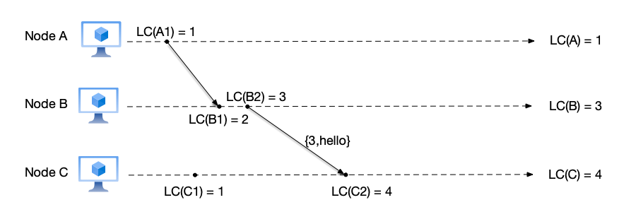
Let us illustrate the calculation process of Lamport clocks through an example. In the figures below, “LC” denotes Lamport Clock, uppercase letters denote node names, and an uppercase letter plus a number denotes the nth event on that node. For example, LC(A) = 1 means that node A’s Lamport clock is currently 1, and LC(A1) = 2 means that the Lamport clock of the first event on node A is 2.

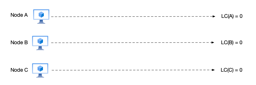
1. Initial state: At this point the Lamport clock values of nodes A, B, and C are all 0, i.e., LC(A) = LC(B) = LC(C) = 0.

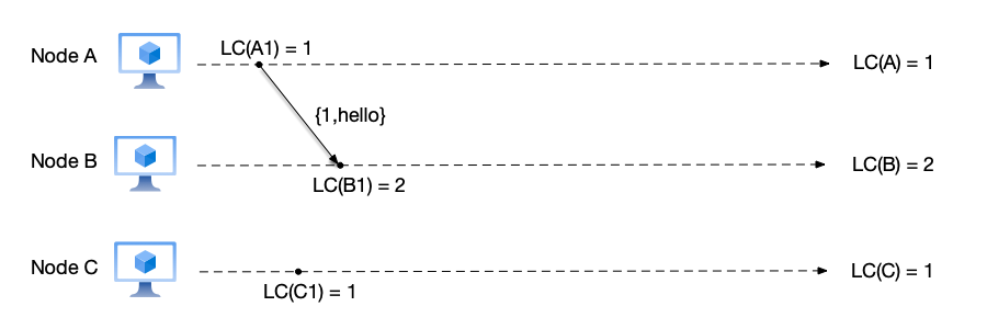
2. Node A sends a message to node B:
   • Node A: before executing the send message event, node A increments its counter to LC(A) = LC(A) + 1 = 1, then sends the current count value as part of the message to node B. Therefore, the logical clock corresponding to this send message event LC(A1) is 1;
   • Node B: after receiving the message from node A, it updates its local counter to LC(B) = max(LC(B), $C_{msg}$) = 1, then increments the counter to LC(B) = LC(B) + 1 = 2. Therefore, the logical clock corresponding to this receive message event LC(B1) is 2;
   • Node C: a local event occurs on node C, LC(C1) = 1.

3. Node B sends a message to node C:
   • Node A: because no new event occurs, node A keeps LC(A) = 1;
   • Node B: before executing the send message event, node B increments its counter to LC(B) = LC(B) + 1 = 3, then sends the current count value as part of the message to node C. Therefore, the logical clock corresponding to this send message event LC(B2) is 3;
   • Node C: after receiving the message from node B, it updates its local counter to LC(C) = max(LC(C), $C_{msg}$) = 3, then increments the counter to LC(C) = LC(C) + 1 = 4. Therefore, the logical clock corresponding to this receive message event LC(C2) is 4.

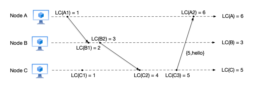
4. Node C sends a message to node A:
   • Node A: after receiving the message from node C, it updates its local counter to LC(A) = max(LC(A), $C_{msg}$) = 5, then increments the counter to LC(A) = LC(A) + 1 = 6. Therefore, the logical clock corresponding to this receive message event LC(A2) is 6;
   • Node B: because no new event occurs, node B keeps LC(B) = 3;
   • Node C: before executing the send message event, node C increments its counter to LC(C) = LC(C) + 1 = 5, then sends the current count value as part of the message to node A. Therefore, the logical clock corresponding to this send message event LC(C3) is 5.

It is easy to see that the calculation rules for Lamport clocks satisfy the clock condition that any logical clock implementation must satisfy. It guarantees the clock condition in the following ways:

• Local events: each time a node executes an event, it increments its local Lamport clock by 1. In this way, events occurring sequentially within the node can reflect their order through the Lamport clock. For example, events B1 and B2 in the earlier figure, LC(B1) = 2 < LC(B2) = 3;
• Message send/receive events: when a node sends a message, it carries the Lamport clock corresponding to that send message in the message body. When receiving a message, it takes the larger of the current local Lamport clock and the message’s Lamport clock, then increments by 1 as the receive event time. For example, events B2 and C2 in the earlier figure are the corresponding message send and receive events, LC(B2) = 3 < LC(C2) = 4.

Conversely, the magnitude of two events’ Lamport clocks cannot reflect their order. For example, in the figure, LC(C1) = 1 < LC(B2) = 3, but these two events are concurrent events.

It can be seen that although Lamport clocks maintain the clock condition required by logical clocks, they cannot determine the causal relationships between events through this time. The vector clock introduced below can solve this problem.

Note: Although the Lamport clock mentioned in this paper does not satisfy the strong consistency condition, this does not prevent the paper from becoming one of the most important papers in the distributed systems field. In addition to proposing the definition of the Happened-before relation and the calculation method of Lamport logical clocks, the paper more importantly proposes that any distributed system can be described as a state machine composed of events in a specific order. If the multiple nodes that make up a distributed system execute the same events in the same order, they can form the same state machine, and what determines the event order is the logical clock mentioned here. This idea is also the foundation of consensus algorithms such as Paxos and Raft mentioned later.

Vector Clocks #

The problem with Lamport clocks is that using a single integer to simultaneously represent both local logical time and global logical time is insufficient for tracking the causal relationships of events. In the earlier figure, the reason why LC(A1) and LC(C1) are both 1 is that from the perspectives of nodes A and C, the local logical time and global logical time they see are both 1.

Vector clocks were proposed by Friedemann Mattern in 1988 [21]. Its idea is: each node has its own local logical time, and the logical times of all nodes together form a vector. This time vector is the global logical time. To synchronize this global logical time, when nodes communicate, in addition to synchronizing their own node’s time value, they also synchronize the time values of other nodes saved on this node. In this way, a globally unique global logical time can be maintained.

Vector clocks can conveniently be used to track the causal history of events. Still taking the earlier figure as an example, the causal history of event C2 is: $\{A1,B1,B2,C1\}$. All events in this set happened before event C2. In addition, vector clocks also satisfy the strong consistency condition: if $VC_i[j] < VC_m[n]$, then there must be $e_{i,j} \to e_{m,n}$; and if two events are concurrent events, it means that the vector clocks of the two events cannot be compared, and vice versa.

---

Let us now introduce the specific implementation of vector clocks. Each node i maintains a clock vector $VC_i$, whose length is the number of nodes in the distributed system, and the initial value of the vector is $[0,\cdots,0]$. $VC_i[j]$ represents the logical time of node j saved on node i, where $i$ and $j$ represent node indices. The calculation rules for vector clocks are as follows:

• Rule 1: before executing an event on node i (events include receiving, sending messages, or local events), increment the logical time of this node by 1, i.e., $VC_i[i] = VC_i[i] + 1$;
• Rule 2: when sending a message, perform operations in the following order:
  • According to rule 1: increment the logical time of this node in the vector clock, i.e., $VC_i[i] = VC_i[i] + 1$;
  • Attach this node’s vector clock $VC_i$ to the message body;
• Rule 3: when receiving a message, perform operations in the following order:
  • Update the local vector clock according to the vector clock in the message. For each component k in the vector, $VC_i[k] = max(VC_i[k], VC_j[k])$;
  • According to rule 1: increment the logical time of this node in the vector clock, i.e., $VC_i[i] = VC_i[i] + 1$.

Because logical clocks are expressed as vectors, we need to define the rules for vector comparison. $VC_i < VC_j$ if and only if the following conditions are satisfied simultaneously:

• For every component k in the vector, $VC_i[k] \leq VC_j[k]$;
• There exists at least one component k such that $VC_i[k] < VC_j[k]$.

For example, $VC_i = [0,1,2] < VC_j = [1,1,2]$, while vectors $[1,2,3]$ and $[1,3,2]$ cannot be compared.

---

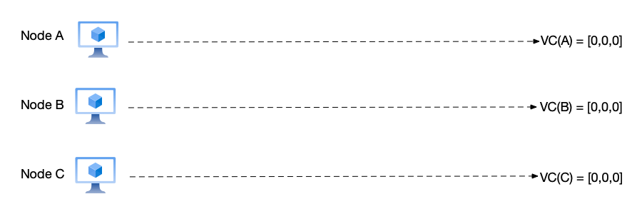
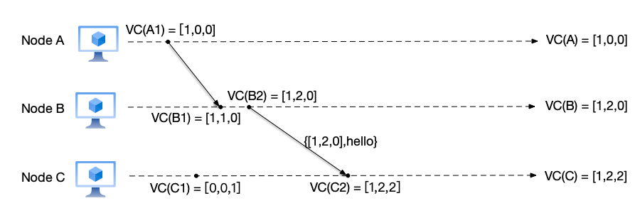
As a comparison, let us re-implement the previous Lamport clock example using vector clocks. In the figures below, “VC” denotes vector clock, uppercase letters denote node names, an uppercase letter plus a number denotes the nth event on that node, and “[k]” denotes taking the kth component value of the vector clock. For example, VC(A) = [1,0,0] means that node A’s current vector clock is [1,0,0], and VC(A1) = [2,0,0] means that the vector clock of the first event on node A is [2,0,0].

1. Initial state: At this point the vector clock values of nodes A, B, and C are all 0, i.e., VC(A) = VC(B) = VC(C) = [0,0,0].

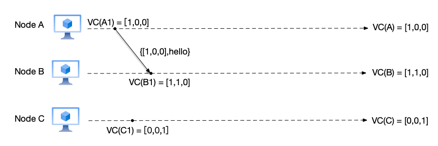
2. Node A sends a message to node B:
   • Node A: before executing the send message event, node A increments the vector counter corresponding to this node in the local vector clock, i.e., $VC(A)[1] = VC(A)[1] + 1 = 1$, obtaining the new vector clock $VC(A) = [1,0,0]$, then sends the current vector clock as part of the message to node B. Therefore, the vector clock corresponding to this send message event VC(A1) is [1,0,0];
   • Node B: after receiving the message from node A, it updates its local vector counter to VC(B)[1] = max(VC(B)[1], $VC_{msg}[1]$) = 1, then increments the local vector clock’s counter for this node to $VC(B)[2] = VC(B)[2] + 1 = 1$. Therefore, the vector clock corresponding to this receive message event VC(B1) is [1,1,0];
   • Node C: a local event occurs on node C, VC(C1) = [0,0,1].

3. Node B sends a message to node C:
   • Node A: because no new event occurs, node A keeps VC(A) = [1,0,0];
   • Node B: before executing the send message event, node B increments its counter to VC(B)[2] = VC(B)[2] + 1 = 2, then sends the current vector clock as part of the message to node C. Therefore, the vector clock corresponding to this send message event VC(B2) is [1,2,0];
   • Node C: after receiving the message from node B, it updates its local vector counter to VC(C)[1] = max(VC(C)[1], $VC_{msg}[1]$) = 1 and VC(C)[2] = max(VC(C)[2], $VC_{msg}[2]$) = 2, then increments its counter to $VC(C)[3] = VC(C)[3] + 1 = 2$. Therefore, the vector clock corresponding to this receive message event VC(C2) is [1,2,2].

4. Node C sends a message to node A:
   • Node A: after receiving the message from node C, it updates its local vector counter: for each component k in the vector, $VC(A)[k] = max(VC(A)[k], VC_{msg}[k])$, thus obtaining $VC(A) = [1,2,3]$, then increments the counter to $VC(A)[1] = VC(A)[1] + 1 = 2$. Therefore, the vector clock corresponding to this receive message event VC(A2) is $[2,2,3]$;
   • Node B: because no new event occurs, node B keeps VC(B) = [1,2,0];
   • Node C: before executing the send message event, node C increments its counter to VC(C)[3] = VC(C)[3] + 1 = 3, then sends the current count value as part of the message to node A. Therefore, the vector clock corresponding to this send message event VC(C3) is [1,2,3].

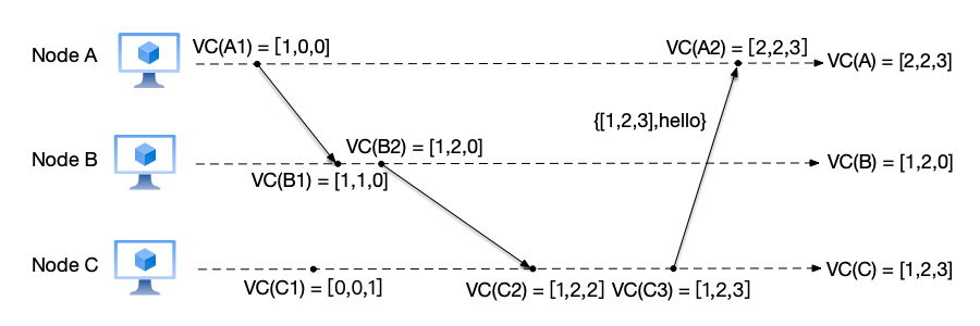
We mentioned earlier that the causal history of event C2 is: $\{A1,B1,B2,C1\}$. All events in the set happened before event C2, because the vector clocks of these events are all smaller than the vector clock of event C2.

In addition, in the earlier Lamport clock figure, LC(C1) = 1 < LC(B2) = 3, but we cannot assert the causal relationship between the two from this. That is, when LC(a) < LC(b), it is possible that event a happened before event b, or the two events may be concurrent events. In the Lamport clock algorithm: $LC(a) < LC(b) \Rightarrow (a \to b) \lor (a \| b)$.

In the vector clock figure, VC(C1) = [0,0,1] and VC(B2) = [1,2,0]. According to the vector clock comparison algorithm, the two cannot be compared in magnitude. Therefore, we can assert that the two events are concurrent events.

Although vector clocks perfectly solve the problem that Lamport clocks cannot identify concurrent events and satisfy the strong consistency condition, there is no such thing as a free lunch. The “perfection” of vector clocks comes at the cost of storage.

We notice that the length of the vector clock $VC$ depends on the number of nodes $N$ in the system. This means:

• Network bandwidth consumption: every message transmission needs to carry this vector of length $N$. If this is in a cluster with hundreds or thousands of nodes, or in a microservices architecture with thousands of service instances, the data volume of this vector may become very large, even exceeding the size of the message body itself, consuming precious network bandwidth.
• Storage space consumption: each node needs to locally maintain and store this ever-growing vector.
• Poor support for dynamics: vector clocks usually assume that the number of nodes in the system is fixed. If the system frequently performs dynamic scaling (nodes going online or offline), maintaining a vector of fixed length will become extremely difficult and inefficient.

Note: We will see how vector clocks are used to guarantee causal ordering between events, and how Amazon’s Dynamo system uses vector clocks to resolve data conflicts.

Global Snapshots in Distributed Systems #

As an application of logical clocks, let us see how to obtain global snapshots in distributed systems.

In distributed systems, snapshots have the following uses:

• Fault recovery and checkpointing: computational tasks in distributed systems usually involve multiple nodes, and depend on non-deterministic inputs (such as network requests). If a system failure occurs, snapshots can save the global state of the system, so that after fault recovery, computation can restart from the nearest checkpoint, avoiding recalculation from scratch and reducing waste of computing resources and data loss.
• Consistency checking and global state capture: the state of a distributed system is scattered across multiple nodes. Snapshots can help capture a globally consistent state of the system. This is very useful for debugging, verifying system behavior, or detecting data consistency. For example, through snapshots, we can check whether distributed transactions meet consistency requirements.
• Deadlock detection: in distributed systems, deadlocks may involve mutual waiting among multiple nodes. Snapshots can capture the state of all nodes in the system, helping to detect whether deadlock situations exist and providing a basis for solving the problem.
• Distributed debugging and performance analysis: snapshots can record the state of a distributed system at a certain moment, helping developers analyze the system’s operating conditions, locate performance bottlenecks, or logical errors.
• Log compaction and state recovery: in distributed systems, logs may be very large. By periodically creating snapshots, logs can be compacted to the snapshot point, reducing the overhead of log storage, and allowing the system state to be quickly rebuilt based on the snapshot and subsequent logs during recovery.
• Distributed algorithm verification: the correctness of certain distributed algorithms (such as consensus algorithms, distributed locks, etc.) depends on the global state of the system. Snapshots can be used to verify whether these algorithms satisfy expected properties during execution.
• Fault tolerance and high availability: snapshots are one of the key technologies for achieving fault tolerance and high availability. By periodically saving system state, services can be quickly recovered in the event of node failures or network partitions, reducing downtime.

---

At the beginning of this chapter, we briefly explained the concepts of state, events, and snapshots. With the definition of the Happened-before relation, we can now give the properties that snapshots need to satisfy:

If $A \to B$, and B is an event saved in the generated snapshot, then event A must also be in snapshot B.

This property requires that snapshots must not have the situation of missing causal history: if an event appears in a snapshot, all events that happened before that event should also appear in the snapshot.

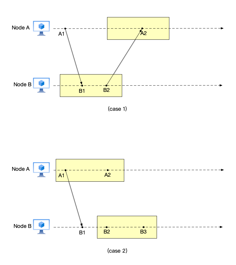
Only snapshots that satisfy this property can be called consistent snapshots. For example, the snapshot below (the snapshot is composed of events within the rectangle) is not a consistent snapshot:

• Case 1: event $A1 \to B1$, and node B’s snapshot has event B1, but event A1 is not in node A’s snapshot;
• Case 2: event $B1 \to B2$, and node B’s snapshot has event B2, but event B1 is not in node B’s snapshot;

Both cases above belong to the missing causal history problem: some event is recorded in the snapshot, but some other events that happened before it are not recorded in the snapshot.

---

If a system runs as a single node, obtaining a snapshot is relatively simple: we only need to obtain the state of all variables and combinations of events on that node at a specific time to generate the snapshot. But when the system runs with multiple nodes, things become complicated: each node has its own state, and events between nodes can affect the node’s state.

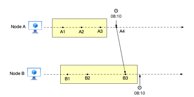
An intuitive way is to use a “global clock” to notify other nodes. After receiving the message, nodes return their state before that time. As introduced earlier, synchronizing between nodes using physical clocks is unreliable. As shown below, node A records its current snapshot (including events $\{A1,A2,A3\}$) at 8:10 and simultaneously sends a message to node B (the send message event is A4), asking node B to record its state. Due to clock skew, node B’s time is only 8:10 after receiving the message, so the receive message event B3 is also recorded in node B’s state. That is, node B’s snapshot consists of events $\{B1,B2,B3\}$. Note that node A’s snapshot does not include event A4, which caused event B3. Therefore, this snapshot is not consistent, because event B3 appears out of nowhere. According to the properties that snapshots need to satisfy mentioned earlier, if event B3 appears in the snapshot, all events that happened before it should be in the snapshot, but event A4 is not in node A’s snapshot, violating the snapshot property. The cause of this problem is using physical time as the basis for recording snapshots.

---

Lamport and Chandy proposed an algorithm for recording global state in distributed systems in their paper [22] (the algorithm is named the Chandy-Lamport algorithm [23] after the two authors).

In the paper, to help readers better understand the algorithm’s idea, Lamport used the example of photographing a flock of birds. When a photographer wants to take a picture of a flock of birds in the sky, because there are so many birds and it is impossible to keep them still during the shot, the photographer’s approach is to take multiple photos and finally stitch these photos into an overall scene. Here, birds can be analogized to nodes in a distributed system.

But the difference between a distributed system and a flock of birds is that nodes in a distributed system send messages to each other to communicate, and these messages may change the node’s state. Therefore, in addition to recording the node’s own state, the algorithm also needs to record the messages received by that node, so that a local snapshot of a node can be obtained. The local snapshots of all nodes in the system together form the global snapshot of the system. In addition, in order not to interfere with the message sending of nodes in the distributed system, the algorithm also defines a Marker message. This message does not change the internal state of nodes and is used to notify nodes of the start and end of recording local snapshots.

Before formally introducing the algorithm steps, we need to solve a tricky problem first: how to record those messages that are currently in flight?

Imagine we are watching a video recording of a soccer match. If at a certain second we press the pause button (snapshot), the positions of all players on the field are frozen (node state). But on the field, there may still be a soccer ball flying in the air (message in transit). It has just been kicked by player A but has not yet been received by player B.

If we only record the positions of the players and do not record this flying soccer ball, then when we resume the match (recover from the snapshot), this ball vanishes into thin air—player A thinks “I already kicked it out,” but player B has not received it, and the system state has lost data. This is obviously wrong.

Therefore, a perfect global snapshot must not only record the positions of all players (node states), but also “capture” all soccer balls flying in the air (channel messages) and put them into the snapshot.

The Chandy-Lamport algorithm cleverly uses Marker messages to solve this problem. The logic is as follows:

• Red line division (consistent cut): imagine the Marker as an invisible red dividing line.
• Before the red line: messages sent before the Marker belong to the “past” and should be included in the snapshot.
• After the red line: messages sent after the Marker belong to the “future” and should not appear in this snapshot.

When node A records its own state and sends out a Marker to node B, node A has already entered the “post-snapshot” world. However, node B has not yet received this Marker; it is still living in the “pre-snapshot” world.

During this time difference (after A sends the Marker, before B receives the Marker), if any message flies from A to B:

• For A, this message is sent after it recorded its state (belongs to the future);
• But for B, is it received before it records its state? No, the algorithm requires B to receive the Marker before it can “freeze.”

Let us look at it from the perspective of the receiver. Suppose node B has already recorded its own state (because it may have first received a Marker from C, triggering the snapshot), but it has not yet received the Marker from A.

At this point, both A and B are in the process of recording the snapshot. If A sent a message m1 to B before sending the Marker, this message m1 obviously belongs to the “past.”

• If m1 arrives before B records its state, B will update its own state (x=x+m1), which is fine.
• Key point: if m1 flies slowly and arrives after B has already recorded its local state (taken the photo), but at this time B has not yet received A’s Marker. This means m1 belongs to “before the red line” (A sent it before sending the Marker), but it missed B’s “photo moment.”

In order not to lose this “late” m1, the algorithm requires: after node B records its own state, it must turn on a video recorder to specifically record all messages coming from A’s channel until it receives A’s Marker. These messages are the “patch data” that “clearly belong to the past but missed the photo due to network delay.”

Understanding that recording channel messages is to capture those late, in-transit messages belonging to the past state, let us look at the specific algorithm flow. The algorithm has the following assumptions:

• Messages between nodes will not be lost and will eventually arrive at the receiver;
• Message channels between nodes are FIFO queues, i.e., messages will not be out of order;
• Message channels on nodes are divided into two types: outbound channels and inbound channels;
• Nodes will not crash.

With the above assumptions, let us look at the algorithm implementation.

1. The node responsible for initializing the snapshot has the following tasks:
   • Record the current state of this node;
   • Broadcast marker messages to other nodes through the outbound channels on this node;
   • Start recording messages received on inbound channels;
2. If a node that has started recording a snapshot receives a message that is not a marker message, it needs to record these messages until it receives a marker message;
3. After a node (including the node responsible for initializing the snapshot) receives a marker message, depending on whether it has received a marker message before, there are different treatments:
   • If it has not received a marker message before:
     • The node starts recording the state on this node;
     • Mark the channel that received the marker message as empty;
     • Broadcast marker messages to other nodes through the outbound channels on this node.
   • If it has received a marker message before, stop recording events from the channel that received the marker message.
4. When all nodes’ inbound channels have received marker messages, it means all nodes have recorded their snapshots. The local snapshots on all nodes will form a global snapshot.

---

Let us use an example to illustrate the operation flow of the Chandy-Lamport algorithm:

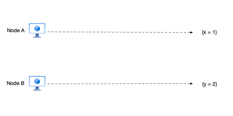
1. Initial state: The system has two nodes A and B, with states $\{x=1\}$ and $\{y=2\}$ respectively.

2. Start recording snapshot: Node A records the current snapshot of this node as $\{x=1\}$, then sends a marker message to node B, notifying it to start recording a snapshot. Before node B receives the marker message, node B also sends a data modification message to node A.

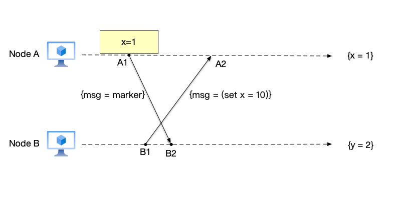
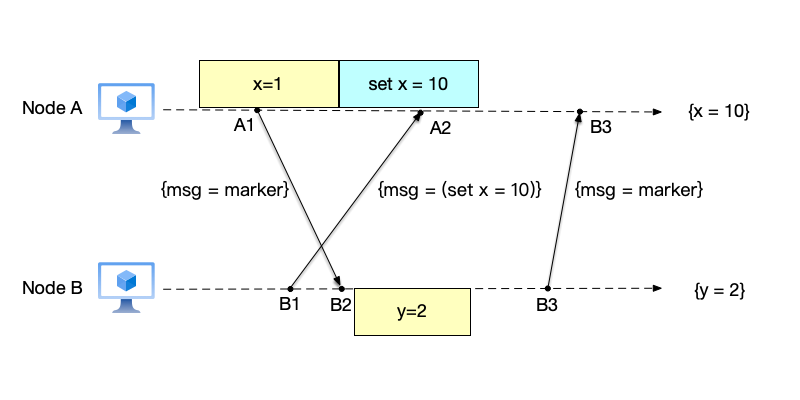
3. Record received non-marker events: Node A receives the data modification message from node B. Since this message is not a marker message, node A needs to record this message. After node B receives the marker message from node A, it needs to record the current snapshot as $\{y=2\}$.

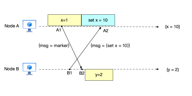
4. Complete global snapshot recording: After recording the snapshot, node B sends a marker message to node A. After node A receives the marker message from node B, it knows that node B has completed its local snapshot. Since there are only two nodes in this system, a global snapshot is generated at this point. The local snapshots are: snapshot $\{x=1\}$ and event $set\ x=10$ on node A, and snapshot $\{y=2\}$ on node B. Together, these local snapshots form the global snapshot $\{x=10,y=2\}$.

Chapter Summary #

In this chapter, we started from the most fundamental yet most confusing concept in distributed systems—“time”—and explored how to determine the order of events in a system without a global clock.

We first recognized that order determines state. If a distributed system is viewed as a state machine, then only by ensuring that each replica executes the same events in the same order can it ultimately reach a consistent state. However, attempting to find this order through physical clocks is unreliable. Whether it is the wall clock or the monotonic clock, limited by the physical characteristics of quartz oscillation, the network asymmetry of the NTP protocol, and the accumulated error of hierarchical synchronization, physical time always has skew and drift during cross-node communication and cannot serve as an absolute measure for determining the order of events.

To break free from the constraints of physical time, we introduced Lamport’s Happened-before relation ($\to$), which is the cornerstone for understanding distributed ordering. It divides the relationships between events into “before” relationships with causality and “concurrent” relationships that cannot be compared. Based on this, we distinguished the two important mathematical concepts of total order and partial order: single-node systems usually satisfy total order, while distributed systems are essentially partial order systems after concurrency is introduced.

In the exploration of logical clocks, we introduced two implementations:

• Lamport clocks: using a simple counter to satisfy the basic clock condition ($a \to b \Rightarrow C(a) < C(b)$). It imposes a total order on all events but loses some causal information and cannot infer event relationships in reverse.
• Vector clocks: by maintaining causal history, it achieves the strong consistency condition ($a \to b \iff V(a) < V(b)$). It can accurately identify concurrent events, but at the cost of storage and network overhead that grows linearly with the number of nodes.

Finally, as an important application of logical clocks, we learned the Chandy-Lamport global snapshot algorithm. This algorithm cleverly uses Marker messages as “dividing lines” between nodes, capturing a globally consistent state (global state) that satisfies causal consistency without stopping the system’s operation (non-blocking). This tells us that a “snapshot” in a distributed system is not the same moment in physical time, but a logically consistent cut.

Through the study of this chapter, we have established a core concept: in distributed systems, causality is more important than physical time.

By understanding “time and order”, we unlock the door to distributed systems. In the following chapters, we will see how these theories are transformed into engineering practice: from data replication between replicas, to resolving concurrent conflicts, to implementing consensus algorithms (such as Paxos and Raft), all of which rely on the foundational theories about “order” established in this chapter.

---

References #

1. Wikipedia: “State machine replication”

2. Wikipedia: “Isidor Isaac Rabi”, Nobel Prize in Physics 1944

3. Wikipedia: “Atomic clock”

4. Wikipedia: “International Atomic Time”

5. Space.com: “Mysterious boost to Earth’s spin will make Aug. 5 one of the shortest days on record”

6. Wikipedia: “Coordinated Universal Time”

7. Wikipedia: “Leap second”

8. Wikipedia: “Unix time”

9. LinkedIn: “2012 Linux Leap Second Bug — A System Design Lesson”

10. Steven Allen: “Planes Will Crash! Things That Leap Seconds Didn’t, and Did, Cause,” 2013

11. Wikipedia: “Network Time Protocol”

12. Cloudflare: “How and Why the Leap Second Affected Cloudflare DNS”

13. Paul R. Johnson and Robert H. Thomas: “RFC 677: Maintenance of Duplicate Databases,” Network Working Group, January 1975.

14. Wikipedia: “Leslie Lamport”

15. Leslie Lamport: “Time, Clocks, and the Ordering of Events in a Distributed System,” Communications of the ACM, volume 21, number 7, pages 558–565, July 1978. doi:10.1145/359545.359563

16. Wikipedia: “Happened-before”

17. Wikipedia: “Partially ordered set”

18. Wikipedia: “Total order”

19. Wikipedia: “Alibi”

20. M. Raynal and M. Singhal: “Logical Time: Capturing Causality in Distributed Systems,” IEEE Computer, volume 29, number 2, pages 49–56, February 1996.

21. Friedemann Mattern: “Virtual Time and Global States of Distributed Systems,” in Proceedings of the Workshop on Parallel and Distributed Algorithms, pages 215–226, North-Holland, 1989.

22. K. Mani Chandy and Leslie Lamport: “Distributed Snapshots: Determining Global States of Distributed Systems,” ACM Transactions on Computer Systems (TOCS), volume 3, number 1, pages 63–75, February 1985.

23. Wikipedia: “Chandy-Lamport algorithm”